BOCS Channel Scalper Indicator - Mean Reversion Alert System# BOCS Channel Scalper Indicator - Mean Reversion Alert System
## WHAT THIS INDICATOR DOES:
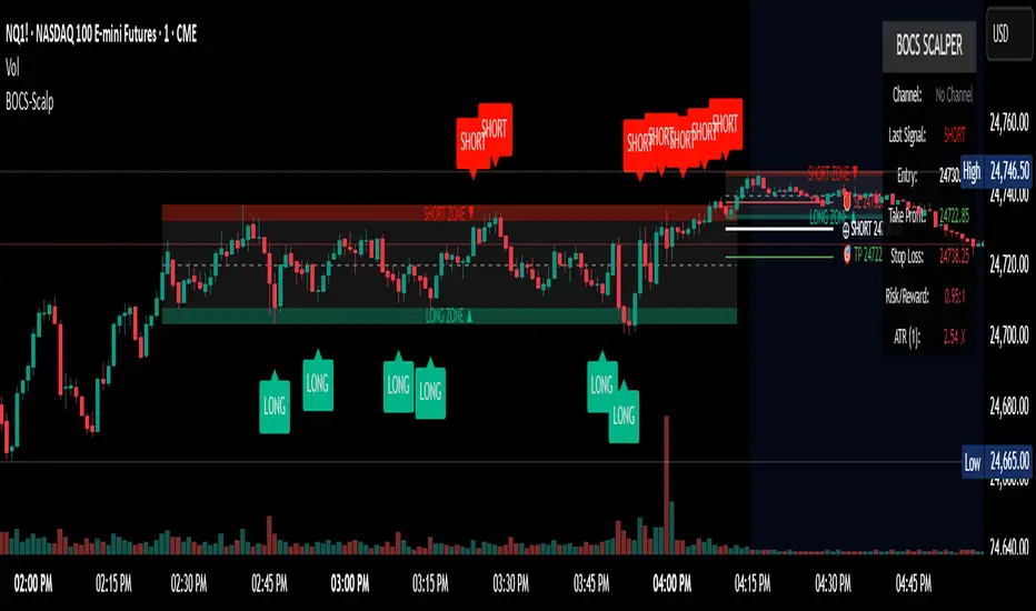
This is a mean reversion trading indicator that identifies consolidation channels through volatility analysis and generates alert signals when price enters entry zones near channel boundaries. **This indicator version is designed for manual trading with comprehensive alert functionality.** Unlike automated strategies, this tool sends notifications (via popup, email, SMS, or webhook) when trading opportunities occur, allowing you to manually review and execute trades. The system assumes price will revert to the channel mean, identifying scalp opportunities as price reaches extremes and preparing to bounce back toward center.
## INDICATOR VS STRATEGY - KEY DISTINCTION:
**This is an INDICATOR with alerts, not an automated strategy.** It does not execute trades automatically. Instead, it:
- Displays visual signals on your chart when entry conditions are met
- Sends customizable alerts to your device/email when opportunities arise
- Shows TP/SL levels for reference but does not place orders
- Requires you to manually enter and exit positions based on signals
- Works with all TradingView subscription levels (alerts included on all plans)
**For automated trading with backtesting**, use the strategy version. For manual control with notifications, use this indicator version.
## ALERT CAPABILITIES:
This indicator includes four distinct alert conditions that can be configured independently:
**1. New Channel Formation Alert**
- Triggers when a fresh BOCS channel is identified
- Message: "New BOCS channel formed - potential scalp setup ready"
- Use this to prepare for upcoming trading opportunities
**2. Long Scalp Entry Alert**
- Fires when price touches the long entry zone
- Message includes current price, calculated TP, and SL levels
- Notification example: "LONG scalp signal at 24731.75 | TP: 24743.2 | SL: 24716.5"
**3. Short Scalp Entry Alert**
- Fires when price touches the short entry zone
- Message includes current price, calculated TP, and SL levels
- Notification example: "SHORT scalp signal at 24747.50 | TP: 24735.0 | SL: 24762.75"
**4. Any Entry Signal Alert**
- Combined alert for both long and short entries
- Use this if you want a single alert stream for all opportunities
- Message: "BOCS Scalp Entry: at "
**Setting Up Alerts:**
1. Add indicator to chart and configure settings
2. Click the Alert (⏰) button in TradingView toolbar
3. Select "BOCS Channel Scalper" from condition dropdown
4. Choose desired alert type (Long, Short, Any, or Channel Formation)
5. Set "Once Per Bar Close" to avoid false signals during bar formation
6. Configure delivery method (popup, email, webhook for automation platforms)
7. Save alert - it will fire automatically when conditions are met
**Alert Message Placeholders:**
Alerts use TradingView's dynamic placeholder system:
- {{ticker}} = Symbol name (e.g., NQ1!)
- {{close}} = Current price at signal
- {{plot_1}} = Calculated take profit level
- {{plot_2}} = Calculated stop loss level
These placeholders populate automatically, creating detailed notification messages without manual configuration.
## KEY DIFFERENCE FROM ORIGINAL BOCS:
**This indicator is designed for traders seeking higher trade frequency.** The original BOCS indicator trades breakouts OUTSIDE channels, waiting for price to escape consolidation before entering. This scalper version trades mean reversion INSIDE channels, entering when price reaches channel extremes and betting on a bounce back to center. The result is significantly more trading opportunities:
- **Original BOCS**: 1-3 signals per channel (only on breakout)
- **Scalper Indicator**: 5-15+ signals per channel (every touch of entry zones)
- **Trade Style**: Mean reversion vs trend following
- **Hold Time**: Seconds to minutes vs minutes to hours
- **Best Markets**: Ranging/choppy conditions vs trending breakouts
This makes the indicator ideal for active day traders who want continuous alert opportunities within consolidation zones rather than waiting for breakout confirmation. However, increased signal frequency also means higher potential commission costs and requires disciplined trade selection when acting on alerts.
## TECHNICAL METHODOLOGY:
### Price Normalization Process:
The indicator normalizes price data to create consistent volatility measurements across different instruments and price levels. It calculates the highest high and lowest low over a user-defined lookback period (default 100 bars). Current close price is normalized using: (close - lowest_low) / (highest_high - lowest_low), producing values between 0 and 1 for standardized volatility analysis.
### Volatility Detection:
A 14-period standard deviation is applied to the normalized price series to measure price deviation from the mean. Higher standard deviation values indicate volatility expansion; lower values indicate consolidation. The indicator uses ta.highestbars() and ta.lowestbars() to identify when volatility peaks and troughs occur over the detection period (default 14 bars).
### Channel Formation Logic:
When volatility crosses from a high level to a low level (ta.crossover(upper, lower)), a consolidation phase begins. The indicator tracks the highest and lowest prices during this period, which become the channel boundaries. Minimum duration of 10+ bars is required to filter out brief volatility spikes. Channels are rendered as box objects with defined upper and lower boundaries, with colored zones indicating entry areas.
### Entry Signal Generation:
The indicator uses immediate touch-based entry logic. Entry zones are defined as a percentage from channel edges (default 20%):
- **Long Entry Zone**: Bottom 20% of channel (bottomBound + channelRange × 0.2)
- **Short Entry Zone**: Top 20% of channel (topBound - channelRange × 0.2)
Long signals trigger when candle low touches or enters the long entry zone. Short signals trigger when candle high touches or enters the short entry zone. Visual markers (arrows and labels) appear on chart, and configured alerts fire immediately.
### Cooldown Filter:
An optional cooldown period (measured in bars) prevents alert spam by enforcing minimum spacing between consecutive signals. If cooldown is set to 3 bars, no new long alert will fire until 3 bars after the previous long signal. Long and short cooldowns are tracked independently, allowing both directions to signal within the same period.
### ATR Volatility Filter:
The indicator includes a multi-timeframe ATR filter to avoid alerts during low-volatility conditions. Using request.security(), it fetches ATR values from a specified timeframe (e.g., 1-minute ATR while viewing 5-minute charts). The filter compares current ATR to a user-defined minimum threshold:
- If ATR ≥ threshold: Alerts enabled
- If ATR < threshold: No alerts fire
This prevents notifications during dead zones where mean reversion is unreliable due to insufficient price movement. The ATR status is displayed in the info table with visual confirmation (✓ or ✗).
### Take Profit Calculation:
Two TP methods are available:
**Fixed Points Mode**:
- Long TP = Entry + (TP_Ticks × syminfo.mintick)
- Short TP = Entry - (TP_Ticks × syminfo.mintick)
**Channel Percentage Mode**:
- Long TP = Entry + (ChannelRange × TP_Percent)
- Short TP = Entry - (ChannelRange × TP_Percent)
Default 50% targets the channel midline, a natural mean reversion target. These levels are displayed as visual lines with labels and included in alert messages for reference when manually placing orders.
### Stop Loss Placement:
Stop losses are calculated just outside the channel boundary by a user-defined tick offset:
- Long SL = ChannelBottom - (SL_Offset_Ticks × syminfo.mintick)
- Short SL = ChannelTop + (SL_Offset_Ticks × syminfo.mintick)
This logic assumes channel breaks invalidate the mean reversion thesis. SL levels are displayed on chart and included in alert notifications as suggested stop placement.
### Channel Breakout Management:
Channels are removed when price closes more than 10 ticks outside boundaries. This tolerance prevents premature channel deletion from minor breaks or wicks, allowing the mean reversion setup to persist through small boundary violations.
## INPUT PARAMETERS:
### Channel Settings:
- **Nested Channels**: Allow multiple overlapping channels vs single channel
- **Normalization Length**: Lookback for high/low calculation (1-500, default 100)
- **Box Detection Length**: Period for volatility detection (1-100, default 14)
### Scalping Settings:
- **Enable Long Scalps**: Toggle long alert generation on/off
- **Enable Short Scalps**: Toggle short alert generation on/off
- **Entry Zone % from Edge**: Size of entry zone (5-50%, default 20%)
- **SL Offset (Ticks)**: Distance beyond channel for stop (1+, default 5)
- **Cooldown Period (Bars)**: Minimum spacing between alerts (0 = no cooldown)
### ATR Filter:
- **Enable ATR Filter**: Toggle volatility filter on/off
- **ATR Timeframe**: Source timeframe for ATR (1, 5, 15, 60 min, etc.)
- **ATR Length**: Smoothing period (1-100, default 14)
- **Min ATR Value**: Threshold for alert enablement (0.1+, default 10.0)
### Take Profit Settings:
- **TP Method**: Choose Fixed Points or % of Channel
- **TP Fixed (Ticks)**: Static distance in ticks (1+, default 30)
- **TP % of Channel**: Dynamic target as channel percentage (10-100%, default 50%)
### Appearance:
- **Show Entry Zones**: Toggle zone labels on channels
- **Show Info Table**: Display real-time indicator status
- **Table Position**: Corner placement (Top Left/Right, Bottom Left/Right)
- **Long Color**: Customize long signal color (default: darker green for readability)
- **Short Color**: Customize short signal color (default: red)
- **TP/SL Colors**: Customize take profit and stop loss line colors
- **Line Length**: Visual length of TP/SL reference lines (5-200 bars)
## VISUAL INDICATORS:
- **Channel boxes** with semi-transparent fill showing consolidation zones
- **Colored entry zones** labeled "LONG ZONE ▲" and "SHORT ZONE ▼"
- **Entry signal arrows** below/above bars marking long/short alerts
- **TP/SL reference lines** with emoji labels (⊕ Entry, 🎯 TP, 🛑 SL)
- **Info table** showing channel status, last signal, entry/TP/SL prices, risk/reward ratio, and ATR filter status
- **Visual confirmation** when alerts fire via on-chart markers synchronized with notifications
## HOW TO USE:
### For 1-3 Minute Scalping with Alerts (NQ/ES):
- ATR Timeframe: "1" (1-minute)
- ATR Min Value: 10.0 (for NQ), adjust per instrument
- Entry Zone %: 20-25%
- TP Method: Fixed Points, 20-40 ticks
- SL Offset: 5-10 ticks
- Cooldown: 2-3 bars to reduce alert spam
- **Alert Setup**: Configure "Any Entry Signal" for combined long/short notifications
- **Execution**: When alert fires, verify chart visuals, then manually place limit order at entry zone with provided TP/SL levels
### For 5-15 Minute Day Trading with Alerts:
- ATR Timeframe: "5" or match chart
- ATR Min Value: Adjust to instrument (test 8-15 for NQ)
- Entry Zone %: 20-30%
- TP Method: % of Channel, 40-60%
- SL Offset: 5-10 ticks
- Cooldown: 3-5 bars
- **Alert Setup**: Configure separate "Long Scalp Entry" and "Short Scalp Entry" alerts if you trade directionally based on bias
- **Execution**: Review channel structure on alert, confirm ATR filter shows ✓, then enter manually
### For 30-60 Minute Swing Scalping with Alerts:
- ATR Timeframe: "15" or "30"
- ATR Min Value: Lower threshold for broader market
- Entry Zone %: 25-35%
- TP Method: % of Channel, 50-70%
- SL Offset: 10-15 ticks
- Cooldown: 5+ bars or disable
- **Alert Setup**: Use "New Channel Formation" to prepare for setups, then "Any Entry Signal" for execution alerts
- **Execution**: Larger timeframes allow more analysis time between alert and entry
### Webhook Integration for Semi-Automation:
- Configure alert webhook URL to connect with platforms like TradersPost, TradingView Paper Trading, or custom automation
- Alert message includes all necessary order parameters (direction, entry, TP, SL)
- Webhook receives structured data when signal fires
- External platform can auto-execute based on alert payload
- Still maintains manual oversight vs full strategy automation
## USAGE CONSIDERATIONS:
- **Manual Discipline Required**: Alerts provide opportunities but execution requires judgment. Not all alerts should be taken - consider market context, trend, and channel quality
- **Alert Timing**: Alerts fire on bar close by default. Ensure "Once Per Bar Close" is selected to avoid false signals during bar formation
- **Notification Delivery**: Mobile/email alerts may have 1-3 second delay. For immediate execution, use desktop popups or webhook automation
- **Cooldown Necessity**: Without cooldown, rapidly touching price action can generate excessive alerts. Start with 3-bar cooldown and adjust based on alert volume
- **ATR Filter Impact**: Enabling ATR filter dramatically reduces alert count but improves quality. Track filter status in info table to understand when you're receiving fewer alerts
- **Commission Awareness**: High alert frequency means high potential trade count. Calculate if your commission structure supports frequent scalping before acting on all alerts
## COMPATIBLE MARKETS:
Works on any instrument with price data including stock indices (NQ, ES, YM, RTY), individual stocks, forex pairs (EUR/USD, GBP/USD), cryptocurrency (BTC, ETH), and commodities. Volume-based features are not included in this indicator version. Multi-timeframe ATR requires higher-tier TradingView subscription for request.security() functionality on timeframes below chart timeframe.
## KNOWN LIMITATIONS:
- **Indicator does not execute trades** - alerts are informational only; you must manually place all orders
- **Alert delivery depends on TradingView infrastructure** - delays or failures possible during platform issues
- **No position tracking** - indicator doesn't know if you're in a trade; you must manage open positions independently
- **TP/SL levels are reference only** - you must manually set these on your broker platform; they are not live orders
- **Immediate touch entry can generate many alerts** in choppy zones without adequate cooldown
- **Channel deletion at 10-tick breaks** may be too aggressive or lenient depending on instrument tick size
- **ATR filter from lower timeframes** requires TradingView Premium/Pro+ for request.security()
- **Mean reversion logic fails** in strong breakout scenarios - alerts will fire but trades may hit stops
- **No partial closing capability** - full position management is manual; you determine scaling out
- **Alerts do not account for gaps** or overnight price changes; morning alerts may be stale
## RISK DISCLOSURE:
Trading involves substantial risk of loss. This indicator provides signals for educational and informational purposes only and does not constitute financial advice. Past performance does not guarantee future results. Mean reversion strategies can experience extended drawdowns during trending markets. Alerts are not guaranteed to be profitable and should be combined with your own analysis. Stop losses may not fill at intended levels during extreme volatility or gaps. Never trade with capital you cannot afford to lose. Consider consulting a licensed financial advisor before making trading decisions. Always verify alerts against current market conditions before executing trades manually.
## ACKNOWLEDGMENT & CREDITS:
This indicator is built upon the channel detection methodology created by **AlgoAlpha** in the "Smart Money Breakout Channels" indicator. Full credit and appreciation to AlgoAlpha for pioneering the normalized volatility approach to identifying consolidation patterns. The core channel formation logic using normalized price standard deviation is AlgoAlpha's original contribution to the TradingView community.
Enhancements to the original concept include: mean reversion entry logic (vs breakout), immediate touch-based alert generation, comprehensive alert condition system with customizable notifications, multi-timeframe ATR volatility filtering, cooldown period for alert management, dual TP methods (fixed points vs channel percentage), visual TP/SL reference lines, and real-time status monitoring table. This indicator version is specifically designed for manual traders who prefer alert-based decision making over automated execution.
Cerca negli script per "stop loss"
Weekend Hunter Ultimate v6.2 Weekend Hunter Ultimate v6.2 - Automated Crypto Weekend Trading System
OVERVIEW:
Specialized trading strategy designed for cryptocurrency weekend markets (Saturday-Sunday) when institutional traders are typically offline and market dynamics differ significantly from weekdays. Optimized for 15-minute timeframe execution with multi-timeframe confluence analysis.
KEY FEATURES:
- Weekend-Only Trading: Automatically activates during configurable weekend hours
- Dynamic Leverage: 5-20x leverage adjusted based on market safety and signal confidence
- Multi-Timeframe Analysis: Combines 4H trend, 1H momentum, and 15M execution
- 10 Pre-configured Crypto Pairs: BTC, ETH, LINK, XRP, DOGE, SOL, AVAX, PEPE, TON, POL
- Position & Risk Management: Max 4 concurrent positions, -30% account protection
- Smart Trailing Stops: Protects profits when approaching targets
RISK MANAGEMENT:
- Maximum daily loss: 5% (configurable)
- Maximum weekend loss: 15% (configurable)
- Per-position risk: Capped at 120-156 USDT
- Emergency stops for flash crashes (8% moves)
- Consecutive loss protection (4 losses = pause)
TECHNICAL INDICATORS:
- CVD (Cumulative Volume Delta) divergence detection
- ATR-based dynamic stop loss and take profit
- RSI, MACD, Bollinger Bands confluence
- Volume surge confirmation (1.5x average)
- Weekend liquidity adjustments
INTEGRATION:
- Designed for Bybit Futures (0.075% taker fee)
- WunderTrading webhook compatibility via JSON alerts
- Minimum position size: 120 USDT (Bybit requirement)
- Initial capital: $500 recommended
TARGET METRICS:
- Win rate target: 65%
- Average win: 5.5%
- Average loss: 1.8%
- Risk-reward ratio: ~3:1
IMPORTANT DISCLAIMERS:
- Past performance does not guarantee future results
- Leveraged trading carries substantial risk of loss
- Weekend crypto markets have 13% of normal liquidity
- Not suitable for traders who cannot afford to lose their entire investment
- Requires continuous monitoring and adjustment
USAGE:
1. Apply to 15-minute charts only
2. Configure weekend hours for your timezone
3. Set up webhook alerts for automation
4. Monitor performance table in top-right corner
5. Adjust parameters based on your risk tolerance
This is an experimental strategy for educational purposes. Always test with small amounts first and never invest more than you can afford to lose completely.

Rachas ATR AssistHey Traders!
This indicator is a simple, it uses Average True Range (ATR) data from the daily chart and the current timeframe to estimate potential range and volatility.
This indicator compares the daily ATR to the current daily wick range (from low to high), helping you gauge how much "room" might be left for price movement within the day. Alongside that, it shows the ATR over the last 14 candles and 5 candles on your current chart for intraday volatility awareness—ideal for setting stops, targets, or position sizing.
Gauge Daily Potential Movement:
The "Day Range Difference" cell shows how much of the expected daily range (based on ATR) is still unfilled. If the market has moved less than the average, there's still potential for expansion. If it's close to or above the ATR, expect a slowdown or reversal.
Position Sizing & Stop Losses:
Use the 14-period ATR and 5-period ATR on your current timeframe to understand recent volatility. This helps in choosing logical stop loss levels and adjusting position sizes based on market conditions.
Volatility Awareness:
Knowing the average daily range and how much of it has been used lets you avoid entering trades too late in the move or placing stops in overly tight spots.
Table Position & Font:
You can adjust the table location (top/bottom left/right) and font size to best fit your chart layout.

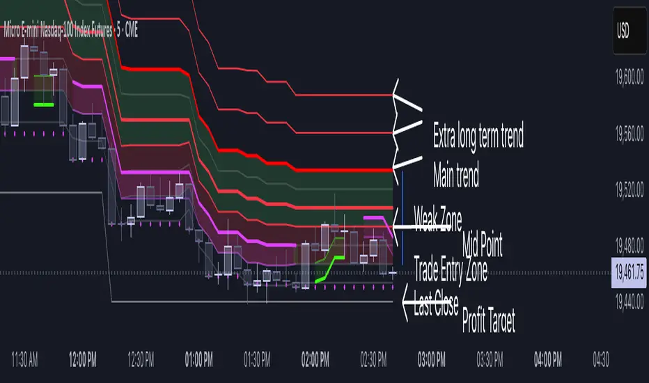
Volatility Layered Supertrend [NLR]We’ve all used Supertrend, but do you know where to actually enter a trade? Volatility Layered Supertrend (VLS) is here to solve that! This advanced trend-following indicator builds on the classic Supertrend by not only identifying trends and their strength but also guiding you to the best trade entry points. VLS divides the main long-term trend into “Strong” and “Weak” Zones, with a clear “Trade Entry Zone” to help you time your trades with precision. With layered trends, dynamic profit targets, and volatility-adaptive bands, VLS delivers actionable signals for any market.
Why I Created VLS Over a Plain Supertrend
I built VLS to address the gaps in traditional Supertrend usage and make trade entries clearer:
Single-Line Supertrend Issues: The default Supertrend sets stop-loss levels that are too wide, making it impractical for most traders to use effectively.
Unclear Entry Points: Standard Supertrend doesn’t tell you where to enter a trade, often leaving you guessing or entering too early or late.
Multi-Line Supertrend Enhancement: Many traders use short, medium, and long Supertrends, which is helpful but can lack focus. In VLS, I include Short, Medium, and Long trends (using multipliers 1 to 3), and add multipliers 4 and 5 to track extra long-term trends—helping to avoid fakeouts that sometimes occur with multiplier 3.
My Solution: I focused on the main long-term Supertrend and split it into “Weak Zone” and “Strength Zone” to show the trend’s reliability. I also defined a “Trade Entry Zone” (starting from the Mid Point, with the first layer’s background hidden for clarity) to guide you on where to enter trades. The zones include Short, Medium, and Long Trend layers for precise entries, exits, and stop-losses.
Practical Trading: This approach provides realistic stop-loss levels, clear entry points, and a “Profit Target” line that aligns with your risk tolerance, while filtering out false signals with longer-term trends.
Key Features
Layered Trend Zones: Short, Medium, Long, and Extra Long Trend layers (up to multipliers 4 and 5) for timing entries and exits.
Strong & Weak Zones: See when the trend is reliable (Strength Zone) or needs caution (Weak Zone).
Trade Entry Zone: A dedicated zone starting from the Mid Point (first layer’s background hidden) to show the best entry points.
Dynamic Profit Targets: A “Profit Target” line that adjusts with the trend for clear goals.
Volatility-Adaptive: Uses ATR to adapt to market conditions, ensuring reliable signals.
Color-Coded: Green for uptrends, red for downtrends—simple and clear.
How It Works
VLS enhances the main long-term Supertrend by dividing it into two zones:
Weak Zone: Indicates a less reliable trend—use tighter stop-losses or wait for the price to reach the Trade Entry Zone.
Strength Zone: Signals a strong trend—ideal for entries with wider stop-losses for bigger moves.
The “Trade Entry Zone” starts at the Mid Point (last layer’s background hidden for clarity), showing you the best area to enter trades. Each zone includes Short, Medium, Long, and Extra Long Trend sublevels (up to multipliers 4 and 5) for precise trade timing and to filter out fakeouts. The “Profit Target” updates dynamically based on trend direction and volatility, giving you a clear goal.
How to Use
Spot the Trend: Green bands = buy, red bands = sell.
Check Strength: Price in Strength Zone? Trend’s reliable—trade confidently. In Weak Zone? Use tighter stops or wait.
Enter Trades: Use the “Trade Entry Zone” (from the Mid Point upward) for the best entry points.
Use Sublevels: Short, Medium, Long, and Extra Long layers in each zone help fine-tune entries and exits.
Set Targets: Follow the Profit Target line for goals—it updates automatically.
Combine Tools: Pair with RSI, MACD, or support/resistance for added confirmation.
Settings
ATR Length: Adjust the ATR period (default 10) to change sensitivity.
Up/Down Colors: Customize colors—green for up, red for down, by default.
Long Term Profitable Swing | AbbasA Story of a Profitable Swing Trading Strategy
Imagine you're sailing across the ocean, looking for the perfect wave to ride. Swing trading is quite similar—you're navigating the stock market, searching for the ideal moments to enter and exit trades. This strategy, created by Abbas, helps you find those waves and ride them effectively to profitable outcomes.
🌊 Finding the Perfect Wave (Entry)
Our journey begins with two simple signs that tell us a great trading opportunity is forming:
- Moving Averages: We use two lines that follow price trends—the faster one (EMA 16) reacts quickly to recent price moves, and the slower one (EMA 30) gives us a longer-term perspective. When the faster line crosses above the slower line, it's like a clear signal saying, "Hey! The wave is rising, and prices might move higher!"
- RSI Momentum: Next, we check a tool called the RSI, which measures momentum (how strongly prices are moving). If the RSI number is above 50, it means there's enough strength behind this rising wave to carry us forward.
When both signals appear together, that's our green light. It's time to jump on our surfboard and start riding this promising wave.
⚓ Safely Riding the Wave (Risk Management)
While we're riding this wave, we want to ensure we're safe from sudden surprises. To do this, we use something called the Average True Range (ATR), which measures how volatile (or bumpy) the price movements are:
- Stop-Loss: To avoid falling too hard, we set a safety line (stop-loss) 8 times the ATR below our entry price. This helps ensure we exit if the wave suddenly turns against us, protecting us from heavy losses.
- Take Profit: We also set a goal to exit the trade at 11 times the ATR above our entry. This way, we capture significant profits when the wave reaches a nice high point.
🌟 Multiple Rides, Bigger Adventures
This strategy allows us to take multiple positions simultaneously—like riding several waves at once, up to 5. Each trade we make uses only 10% of our trading capital, keeping risks manageable and giving us multiple opportunities to win big.
🗺️ Easy to Follow Settings
Here are the basic settings we use:
- Fast EMA**: 16
- Slow EMA**: 30
- RSI Length**: 9
- RSI Threshold**: 50
- ATR Length**: 21
- ATR Stop-Loss Multiplier**: 8
- ATR Take-Profit Multiplier**: 11
These settings are flexible—you can adjust them to better suit different markets or your personal trading style.
🎉 Riding the Waves of Success
This simple yet powerful swing trading approach helps you confidently enter trades, clearly know when to exit, and effectively manage your risk. It’s a reliable way to ride market waves, capture profits, and minimize losses.
Happy trading, and may you find many profitable waves to ride! 🌊✨
Please test, and take into account that it depends on taking multiple longs within the swing, and you only get to invest 25/30% of your equity.

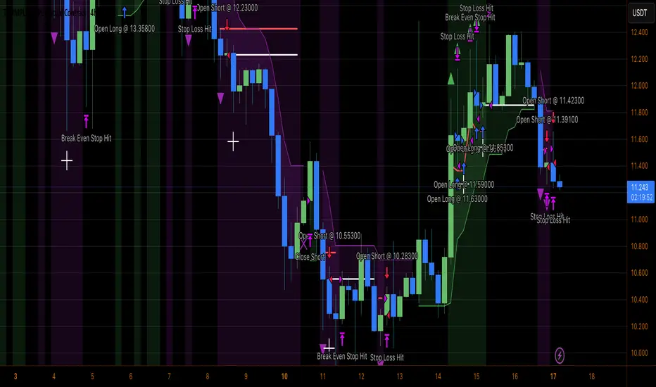
Heiken Ashi Supertrend ATR-SL StrategyThis indicator combines Heikin Ashi candle pattern analysis with Supertrend to generate high-probability trading signals with built-in risk management. It identifies potential entries and exits based on specific Heikin Ashi candlestick formations while providing automated ATR-based stop loss management.
Trading Logic:
The system generates long signals when a green Heikin Ashi candle forms with no bottom wick (indicating strong bullish momentum). Short signals appear when a red Heikin Ashi candle forms with no top wick (showing strong bearish momentum). The absence of wicks on these candles signals a high-conviction market move in the respective direction.
Exit signals are triggered when:
1. An opposite pattern forms (red candle with no top wick exits longs; green candle with no bottom wick exits shorts)
2. The ATR-based stop loss is hit
3. The break-even stop is activated and then hit
Technical Approach:
- Select Heiken Ashi Canldes on your Trading View chart. Entried are based on HA prices.
- Supertrend and ATR-based stop losses use real price data (not HA values) for trend determination
- ATR-based stop losses automatically adjust to market volatility
- Break-even functionality moves the stop to entry price once price moves a specified ATR multiple in your favor
Risk Management:
- Default starting capital: 1000 units
- Default risk per trade: 10% of equity (customizable in strategy settings)
- Hard Stop Loss: Set ATR multiplier (default: 2.0) for automatic stop placement
- Break Even: Configure ATR threshold (default: 1.0) to activate break-even stops
- Appropriate position sizing relative to equity and stop distance
Customization Options:
- Supertrend Settings:
- Enable/disable Supertrend filtering (trade only in confirmed trend direction)
- Adjust Factor (default: 3.0) to change sensitivity
- Modify ATR Period (default: 10) to adapt to different timeframes
Visual Elements:
- Green triangles for long entries, blue triangles for short entries
- X-marks for exits and stop loss hits
- Color-coded position background (green for long, blue for short)
- Clearly visible stop loss lines (red for hard stop, white for break-even)
- Comprehensive position information label with entry price and stop details
Implementation Notes:
The indicator tracks positions internally and maintains state across bars to properly manage stop levels. All calculations use confirmed bars only, with no repainting or lookahead bias. The system is designed for swing trading on timeframes from 1-hour and above, where Heikin Ashi patterns tend to be more reliable.
This indicator is best suited for traders looking to combine the pattern recognition strengths of Heikin Ashi candles with the trend-following capabilities of Supertrend, all while maintaining disciplined risk management through automated stops.
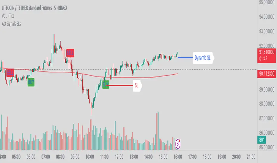
AO Smart Scalper – 5M Dynamic SL Edition📈 AO Signals with Fixed and Dynamic SL – Optimized for 5-Minute Charts 📉
This indicator is built for 5-minute timeframe trading, combining powerful momentum signals from the Awesome Oscillator (AO) with both Fixed and Dynamic Stop Loss (SL) levels to enhance trade management and risk control.
✅ Buy/Sell Signals:
The indicator generates clear BUY and SELL signals based on the AO crossing above or below the zero line, helping traders capture momentum shifts early.
🛑 Fixed Stop Loss:
Each trade signal comes with a Fixed SL, calculated based on the high (for shorts) or low (for longs) of the previous candle, with a customizable percentage offset. This SL is plotted with a red line, providing a clear initial risk level.
⚡ Dynamic Stop Loss: Continuous Presence, Strategic Use:
A secondary Dynamic SL line is plotted, which is continuously present on the chart. This dynamic level responds to market conditions and can serve as a trailing stop or key decision point.
💡 Recommended Use: It is recommended to actively start using the Dynamic SL once the trade has moved into profit. This allows protecting obtained profits and minimizing the risk of losses in case of a market reversal.
🛡️ Enhanced Dynamic Stop-Loss Strategy:
🔒 Initial Protection: Utilize the Fixed SL as the initial stop-loss, placed below relevant lows (for longs) or above relevant highs (for shorts), or as provided by the fixed SL indicator.
🛤️ Dynamic Tracking:
🟢 Long Trades: Once in profit, the Dynamic SL will dynamically adjust, moving upwards as higher lows are formed, effectively trailing the price and securing profits.
🔴 Short Trades: Conversely, in short trades, once in profit, the Dynamic SL will move downwards as lower highs are formed, protecting gains.
🔄 Alternatively the dynamic stop loss will follow the dynamic SL line provided by the indicator.
🚪 Exiting Trades: When the price crosses below the Dynamic SL line in a LONG trade, or above it in a SHORT trade, the recommended action is to exit the trade.
↩️ Re-entry Consideration: You may consider re-entering only if the price clearly returns above the Dynamic SL (for longs) or below it (for shorts).
⚠️ IMPORTANT - 5-Minute Strategy Guidance ⏱️
This tool is specifically optimized for the 5-minute timeframe. This approach helps filter out weak setups and maintain discipline in volatile market conditions.
✨ Additional Features:
👁️ Visual and editable SL levels
📊 200-period SMA for trend context
💻 Simple and effective interface for intraday trading setups
🎯 Ideal for traders seeking a clean, rule-based system that combines momentum entry signals with layered stop loss protection.
🔑 Key Changes:
It was emphasized that the Dynamic SL is always present, but its active use is recommended once the trade is in profit.
It was clarified the use of the Fixed SL, giving the option to use the one provided by the indicator, or to place it according to the price action.
*Auto Backtest & Optimize EngineFull-featured Engine for Automatic Backtesting and parameter optimization. Allows you to test millions of different combinations of stop-loss and take profit parameters, including on any connected indicators.
⭕️ Key Futures
Quickly identify the optimal parameters for your strategy.
Automatically generate and test thousands of parameter combinations.
A simple Genetic Algorithm for result selection.
Saves time on manual testing of multiple parameters.
Detailed analysis, sorting, filtering and statistics of results.
Detailed control panel with many tooltips.
Display of key metrics: Profit, Win Rate, etc..
Comprehensive Strategy Score calculation.
In-depth analysis of the performance of different types of stop-losses.
Possibility to use to calculate the best Stop-Take parameters for your position.
Ability to test your own functions and signals.
Customizable visualization of results.
Flexible Stop-Loss Settings:
• Auto ━ Allows you to test all types of Stop Losses at once(listed below).
• S.VOLATY ━ Static stop based on volatility (Fixed, ATR, STDEV).
• Trailing ━ Classic trailing stop following the price.
• Fast Trail ━ Accelerated trailing stop that reacts faster to price movements.
• Volatility ━ Dynamic stop based on volatility indicators.
• Chandelier ━ Stop based on price extremes.
• Activator ━ Dynamic stop based on SAR.
• MA ━ Stop based on moving averages (9 different types).
• SAR ━ Parabolic SAR (Stop and Reverse).
Advanced Take-Profit Options:
• R:R: Risk/Reward ━ sets TP based on SL size.
• T.VOLATY ━ Calculation based on volatility indicators (Fixed, ATR, STDEV).
Testing Modes:
• Stops ━ Cyclical stop-loss testing
• Pivot Point Example ━ Example of using pivot points
• External Example ━ Built-in example how test functions with different parameters
• External Signal ━ Using external signals
⭕️ Usage
━ First Steps:
When opening, select any point on the chart. It will not affect anything until you turn on Manual Start mode (more on this below).
The chart will immediately show the best results of the default Auto mode. You can switch Part's to try to find even better results in the table.
Now you can display any result from the table on the chart by entering its ID in the settings.
Repeat steps 3-4 until you determine which type of Stop Loss you like best. Then set it in the settings instead of Auto mode.
* Example: I flipped through 14 parts before I liked the first result and entered its ID so I could visually evaluate it on the chart.
Then select the stop loss type, choose it in place of Auto mode and repeat steps 3-4 or immediately follow the recommendations of the algorithm.
Now the Genetic Algorithm at the bottom right will prompt you to enter the Parameters you need to search for and select even better results.
Parameters must be entered All at once before they are updated. Enter recommendations strictly in fields with the same names.
Repeat steps 5-6 until there are approximately 10 Part's left or as you like. And after that, easily pour through the remaining Parts and select the best parameters.
━ Example of the finished result.
━ Example of use with Takes
You can also test at the same time along with Take Profit. In this example, I simply enabled Risk/Reward mode and immediately specified in the TP field Maximum RR, Minimum RR and Step. So in this example I can test (3-1) / 0.1 = 20 Takes of different sizes. There are additional tips in the settings.
━
* Soon you will start to understand how the system works and things will become much easier.
* If something doesn't work, just reset the engine settings and start over again.
* Use the tips I have left in the settings and on the Panel.
━ Details:
Sort ━ Sorting results by Score, Profit, Trades, etc..
Filter ━ Filtring results by Score, Profit, Trades, etc..
Trade Type ━ Ability to disable Long\Short but only from statistics.
BackWin ━ Backtest Window Number of Candle the script can test.
Manual Start ━ Enabling it will allow you to call a Stop from a selected point. which you selected when you started the engine.
* If you have a real open position then this mode can help to save good Stop\Take for it.
1 - 9 Сheckboxs ━ Allow you to disable any stop from Auto mode.
Ex Source - Allow you to test Stops/Takes from connected indicators.
Connection guide:
//@version=6
indicator("My script")
rsi = ta.rsi(close, 14)
buy = not na(rsi) and ta.crossover (rsi, 40) // OS = 40
sell = not na(rsi) and ta.crossunder(rsi, 60) // OB = 60
Signal = buy ? +1 : sell ? -1 : 0
plot(Signal, "🔌Connector🔌", display = display.none)
* Format the signal for your indicator in a similar style and then select it in Ex Source.
⭕️ How it Works
Hypothesis of Uniform Distribution of Rare Elements After Mixing.
'This hypothesis states that if an array of N elements contains K valid elements, then after mixing, these valid elements will be approximately uniformly distributed.'
'This means that in a random sample of k elements, the proportion of valid elements should closely match their proportion in the original array, with some random variation.'
'According to the central limit theorem, repeated sampling will result in an average count of valid elements following a normal distribution.'
'This supports the assumption that the valid elements are evenly spread across the array.'
'To test this hypothesis, we can conduct an experiment:'
'Create an array of 1,000,000 elements.'
'Select 1,000 random elements (1%) for validation.'
'Shuffle the array and divide it into groups of 1,000 elements.'
'If the hypothesis holds, each group should contain, on average, 1~ valid element, with minor variations.'
* I'd like to attach more details to My hypothesis but it won't be very relevant here. Since this is a whole separate topic, I will leave the minimum part for understanding the engine.
Practical Application
To apply this hypothesis, I needed a way to generate and thoroughly mix numerous possible combinations. Within Pine, generating over 100,000 combinations presents significant challenges, and storing millions of combinations requires excessive resources.
I developed an efficient mechanism that generates combinations in random order to address these limitations. While conventional methods often produce duplicates or require generating a complete list first, my approach guarantees that the first 10% of possible combinations are both unique and well-distributed. Based on my hypothesis, this sampling is sufficient to determine optimal testing parameters.
Most generators and randomizers fail to accommodate both my hypothesis and Pine's constraints. My solution utilizes a simple Linear Congruential Generator (LCG) for pseudo-randomization, enhanced with prime numbers to increase entropy during generation. I pre-generate the entire parameter range and then apply systematic mixing. This approach, combined with a hybrid combinatorial array-filling technique with linear distribution, delivers excellent generation quality.
My engine can efficiently generate and verify 300 unique combinations per batch. Based on the above, to determine optimal values, only 10-20 Parts need to be manually scrolled through to find the appropriate value or range, eliminating the need for exhaustive testing of millions of parameter combinations.
For the Score statistic I applied all the same, generated a range of Weights, distributed them randomly for each type of statistic to avoid manual distribution.
Score ━ based on Trade, Profit, WinRate, Profit Factor, Drawdown, Sharpe & Sortino & Omega & Calmar Ratio.
⭕️ Notes
For attentive users, a little tricks :)
To save time, switch parts every 3 seconds without waiting for it to load. After 10-20 parts, stop and wait for loading. If the pause is correct, you can switch between the rest of the parts without loading, as they will be cached. This used to work without having to wait for a pause, but now it does slower. This will save a lot of time if you are going to do a deeper backtest.
Sometimes you'll get the error “The scripts take too long to execute.”
For a quick fix you just need to switch the TF or Ticker back and forth and most likely everything will load.
The error appears because of problems on the side of the site because the engine is very heavy. It can also appear if you set too long a period for testing in BackWin or use a heavy indicator for testing.
Manual Start - Allow you to Start you Result from any point. Which in turn can help you choose a good stop-stick for your real position.
* It took me half a year from idea to current realization. This seems to be one of the few ways to build something automatic in backtest format and in this particular Pine environment. There are already better projects in other languages, and they are created much easier and faster because there are no limitations except for personal PC. If you see solutions to improve this system I would be glad if you share the code. At the moment I am tired and will continue him not soon.
Also You can use my previosly big Backtest project with more manual settings(updated soon)

Smart MA Crossover BacktesterSmart MA Crossover Backtester - Strategy Overview
Strategy Name: Smart MA Crossover Backtester
Published on: TradingView
Applicable Markets: Works well on crypto (tested profitably on ETH)
Strategy Concept
The Smart MA Crossover Backtester is an improved Moving Average (MA) crossover strategy that incorporates a trend filter and an ATR-based stop loss & take profit mechanism for better risk management. It aims to capture trends efficiently while reducing false signals by only trading in the direction of the long-term trend.
Core Components & Logic
Moving Averages (MA) for Entry Signals
Fast Moving Average (9-period SMA)
Slow Moving Average (21-period SMA)
A trade signal is generated when the fast MA crosses the slow MA.
Trend Filter (200-period SMA)
Only enters long positions if price is above the 200-period SMA (bullish trend).
Only enters short positions if price is below the 200-period SMA (bearish trend).
This helps in avoiding counter-trend trades, reducing whipsaws.
ATR-Based Stop Loss & Take Profit
Uses the Average True Range (ATR) with a multiplier of 2 to calculate stop loss.
Risk-Reward Ratio = 1:2 (Take profit is set at 2x ATR).
This ensures dynamic stop loss and take profit levels based on market volatility.
Trading Rules
✅ Long Entry (Buy Signal):
Fast MA (9) crosses above Slow MA (21)
Price is above the 200 MA (bullish trend filter active)
Stop Loss: Below entry price by 2× ATR
Take Profit: Above entry price by 4× ATR
✅ Short Entry (Sell Signal):
Fast MA (9) crosses below Slow MA (21)
Price is below the 200 MA (bearish trend filter active)
Stop Loss: Above entry price by 2× ATR
Take Profit: Below entry price by 4× ATR
Why This Strategy Works Well for Crypto (ETH)?
🔹 Crypto markets are highly volatile – ATR-based stop loss adapts dynamically to market conditions.
🔹 Long-term trend filter (200 MA) ensures trading in the dominant direction, reducing false signals.
🔹 Risk-reward ratio of 1:2 allows for profitable trades even with a lower win rate.
This strategy has been tested on Ethereum (ETH) and has shown profitable performance, making it a strong choice for crypto traders looking for trend-following setups with solid risk management. 🚀

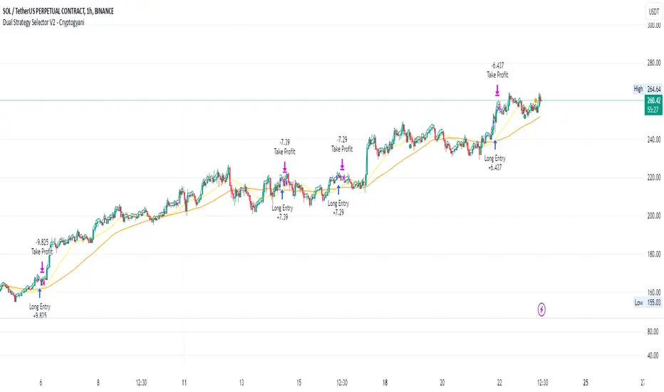
Dual Strategy Selector V2 - CryptogyaniOverview:
This script provides traders with a dual-strategy system that they can toggle between using a simple dropdown menu in the input settings. It is designed to cater to different trading styles and needs, offering both simplicity and advanced filtering techniques. The strategies are built around moving average crossovers, enhanced by configurable risk management tools like take profit levels, trailing stops, and ATR-based stop-loss.
Key Features:
Two Strategies in One Script:
Strategy 1: A classic moving average crossover strategy for identifying entry signals based on trend reversals. Includes user-defined take profit and trailing stop-loss options for profit locking.
Strategy 2: An advanced trend-following system that incorporates:
A higher timeframe trend filter to confirm entry signals.
ATR-based stop-loss for dynamic risk management.
Configurable partial take profit to secure gains while letting the trade run.
Highly Customizable:
All key parameters such as SMA lengths, take profit levels, ATR multiplier, and timeframe for the trend filter are adjustable via the input settings.
Dynamic Toggle:
Traders can switch between Strategy 1 and Strategy 2 with a single dropdown, allowing them to adapt the strategy to market conditions.
How It Works:
Strategy 1:
Entry Logic: A long trade is triggered when the fast SMA crosses above the slow SMA.
Exit Logic: The trade exits at either a user-defined take profit level (percentage or pips) or via an optional trailing stop that dynamically adjusts based on price movement.
Strategy 2:
Entry Logic: Builds on the SMA crossover logic but adds a higher timeframe trend filter to align trades with the broader market direction.
Risk Management:
ATR-Based Stop-Loss: Protects against adverse moves with a volatility-adjusted stop-loss.
Partial Take Profit: Allows traders to secure a percentage of gains while keeping some exposure for extended trends.
How to Use:
Select Your Strategy:
Use the dropdown in the input settings to choose Strategy 1 or Strategy 2.
Configure Parameters:
Adjust SMA lengths, take profit, and risk management settings to align with your trading style.
For Strategy 2, specify the higher timeframe for trend filtering.
Deploy and Monitor:
Apply the script to your preferred asset and timeframe.
Use the backtest results to fine-tune settings for optimal performance.
Why Choose This Script?:
This script stands out due to its dual-strategy flexibility and enhanced features:
For beginners: Strategy 1 provides a simple yet effective trend-following system with minimal setup.
For advanced traders: Strategy 2 includes powerful tools like trend filters and ATR-based stop-loss, making it ideal for challenging market conditions.
By combining simplicity with advanced features, this script offers something for everyone while maintaining full transparency and user customization.
Default Settings:
Strategy 1:
Fast SMA: 21, Slow SMA: 49
Take Profit: 7% or 50 pips
Trailing Stop: Optional (disabled by default)
Strategy 2:
Fast SMA: 20, Slow SMA: 50
ATR Multiplier: 1.5
Partial Take Profit: 50%
Higher Timeframe: 1 Day (1D)
Triple EMA Crossover StrategyTriple EMA Crossover Strategy
Overview
The Triple EMA Crossover Strategy is a trend-following trading system that utilizes three Exponential Moving Averages (EMAs) to identify potential entry and exit points in the market. This strategy is based on the principle that when shorter-term prices cross above longer-term prices, it can indicate a bullish trend, and conversely when they cross below, it can signal a bearish trend.
Components
Exponential Moving Averages (EMAs):
Short EMA: A fast-moving average that reacts quickly to price changes (commonly set to 9 periods).
Medium EMA: A medium-term average that smooths out price data and helps confirm trends (commonly set to 21 periods).
Long EMA: A slow-moving average that helps identify the overall trend direction (commonly set to 55 periods).
Trading Signals:
Buy Signal: A long entry is triggered when:
The Short EMA (9) crosses above the Medium EMA (21).
The Medium EMA (21) is above the Long EMA (55).
Sell Signal: A short entry is signaled when:
The Short EMA (9) crosses below the Medium EMA (21).
The Medium EMA (21) is below the Long EMA (55).
Stop Loss and Take Profit:
Stop Loss: Implement a predefined percentage or ATR-based stop loss to limit potential losses.
Take Profit: Set a target based on a risk-to-reward ratio that reflects your trading strategy's goals.
Advantages
Trend Identification: The EMA crossover system allows traders to identify the current trend dynamically, focusing on upward or downward price movements.
Simplicity: The strategy is straightforward, making it accessible for both new and experienced traders.
Flexibility: This method can be applied across multiple timeframes and asset classes, making it versatile for various trading styles.
Disadvantages
Lagging Indicator: Moving averages are lagging indicators, meaning signals may come later than the actual price movement, which can lead to missed opportunities.
Whipsaw Effect: In ranging markets, the strategy may produce false signals leading to potential losses.
ETH Signal 15m
This strategy uses the Supertrend indicator combined with RSI to generate buy and sell signals, with stop loss (SL) and take profit (TP) conditions based on ATR (Average True Range). Below is a detailed explanation of each part:
1. General Information BINANCE:ETHUSDT.P
Strategy Name: "ETH Signal 15m"
Designed for use on the 15-minute time frame for the ETH pair.
Default capital allocation is 15% of total equity for each trade.
2. Backtest Period
start_time and end_time: Define the start and end time of the backtest period.
start_time = 2024-08-01: Start date of the backtest.
end_time = 2054-01-01: End date of the backtest.
The strategy will only run when the current time falls within this specified range.
3. Supertrend Indicator
Supertrend is a trend-following indicator that provides buy or sell signals based on the direction of price changes.
factor = 2.76: The multiplier used in the Supertrend calculation (increasing this value makes the Supertrend less sensitive to price movements).
atrPeriod = 12: Number of periods used to calculate ATR.
Output:
direction: Determines the buy/sell direction based on Supertrend.
If direction decreases, it signals a buy (Long).
If direction increases, it signals a sell (Short).
4. RSI Indicator
RSI (Relative Strength Index) is a momentum indicator, often used to identify overbought or oversold conditions.
rsiLength = 12: Number of periods used to calculate RSI.
rsiOverbought = 70: RSI level considered overbought.
rsiOversold = 30: RSI level considered oversold.
5. Entry Conditions
Long Entry:
Supertrend gives a buy signal (ta.change(direction) < 0).
RSI must be below the overbought level (rsi < rsiOverbought).
Short Entry:
Supertrend gives a sell signal (ta.change(direction) > 0).
RSI must be above the oversold level (rsi > rsiOversold).
The strategy will only execute trades if the current time is within the backtest period (in_date_range).
6. Stop Loss (SL) and Take Profit (TP) Conditions
ATR (Average True Range) is used to calculate the distance for Stop Loss and Take Profit based on price volatility.
atr = ta.atr(atrPeriod): ATR is calculated using 12 periods.
Stop Loss and Take Profit are calculated as follows:
Long Trade:
Stop Loss: Set at close - 4 * atr (current price minus 4 times the ATR).
Take Profit: Set at close + 2 * atr (current price plus 2 times the ATR).
Short Trade:
Stop Loss: Set at close + 4 * atr (current price plus 4 times the ATR).
Take Profit: Set at close - 2.237 * atr (current price minus 2.237 times the ATR).
Summary:
This strategy enters a Long trade when the Supertrend indicates an upward trend and RSI is not in the overbought region. Conversely, a Short trade is entered when Supertrend signals a downtrend, and RSI is not oversold.
The trade is exited when the price reaches the Stop Loss or Take Profit levels, which are determined based on price volatility (ATR).
Disclaimer:
The content provided in this strategy is for informational and educational purposes only. It is not intended as financial, investment, or trading advice. Trading in cryptocurrency, stocks, or any financial markets involves significant risk, and you may lose more than your initial investment. Past performance is not indicative of future results, and no guarantee of profit can be made. You should consult with a professional financial advisor before making any investment decisions. The creator of this strategy is not responsible for any financial losses or damages incurred as a result of following this strategy. All trades are executed at your own risk.

Fractal Breakout Trend Following StrategyOverview
The Fractal Breakout Trend Following Strategy is a trend-following system which utilizes the Willams Fractals and Alligator to execute the long trades on the fractal's breakouts which have a high probability to be the new uptrend phase beginning. This system also uses the normalized Average True Range indicator to filter trades after a large moves, because it's more likely to see the trend continuation after a consolidation period. Strategy can execute only long trades.
Unique Features
Trend and volatility filtering system: Strategy uses Williams Alligator to filter the counter-trend fractals breakouts and normalized Average True Range to avoid the trades after large moves, when volatility is high
Configurable Trading Periods: Users can tailor the strategy to specific market windows, adapting to different market conditions.
Flexible Risk Management: Users can choose the stop-loss percent (by default = 3%) for trades, but strategy also has the dynamic stop-loss level using down fractals.
Methodology
The strategy places stop order at the last valid fractal breakout level. Validity of this fractal is defined by the Williams Alligator indicator. If at the moment of time when price breaking the last fractal price is higher than Alligator's teeth line (8 period SMA shifted 5 bars in the future) this is a valid breakout. Moreover strategy has the additional volatility filtering system using normalized ATR. It calculates the average normalized ATR for last user-defined number of bars and if this value lower than the user-defined threshold value the long trade is executed.
When trade is opened, script places the stop loss at the price higher of two levels: user defined stop-loss from the position entry price or down fractal validation level. The down fractal is valid with the rule, opposite as the up fractal validation. Price shall break to the downside the last down fractal below the Willians Alligator's teeth line.
Strategy has no fixed take profit. Exit level changes with the down fractal validation level. If price is in strong uptrend trade is going to be active until last down fractal is not valid. Strategy closes trade when price hits the down fractal validation level.
Risk Management
The strategy employs a combined approach to risk management:
It allows positions to ride the trend as long as the price continues to move favorably, aiming to capture significant price movements. It features a user-defined stop-loss parameter to mitigate risks based on individual risk tolerance. By default, this stop-loss is set to a 3% drop from the entry point, but it can be adjusted according to the trader's preferences.
Justification of Methodology
This strategy leverages Williams Fractals to open long trade when price has broken the key resistance level to the upside. This resistance level is the last up fractal and is shall be broken above the Williams Alligator's teeth line to be qualified as the valid breakout according to this strategy. The Alligator filtering increases the probability to avoid the false breakouts against the current trend.
Moreover strategy has an additional filter using Average True Range(ATR) indicator. If average value of ATR for the last user-defined number of bars is lower than user-defined threshold strategy can open the long trade according to open trade condition above. The logic here is following: we want to open trades after period of price consolidation inside the range because before and after a big move price is more likely to be in sideways, but we need a trend move to have a profit.
Another one important feature is how the exit condition is defined. On the one hand, strategy has the user-defined stop-loss (3% below the entry price by default). It's made to give users the opportunity to restrict their losses according to their risk-tolerance. On the other hand, strategy utilizes the dynamic exit level which is defined by down fractal activation. If we assume the breaking up fractal is the beginning of the uptrend, breaking down fractal can be the start of downtrend phase. We don't want to be in long trade if there is a high probability of reversal to the downside. This approach helps to not keep open trade if trend is not developing and hold it if price continues going up.
Backtest Results
Operating window: Date range of backtests is 2023.01.01 - 2024.05.01. It is chosen to let the strategy to close all opened positions.
Commission and Slippage: Includes a standard Binance commission of 0.1% and accounts for possible slippage over 5 ticks.
Initial capital: 10000 USDT
Percent of capital used in every trade: 30%
Maximum Single Position Loss: -3.19%
Maximum Single Profit: +24.97%
Net Profit: +3036.90 USDT (+30.37%)
Total Trades: 83 (28.92% win rate)
Profit Factor: 1.953
Maximum Accumulated Loss: 963.98 USDT (-8.29%)
Average Profit per Trade: 36.59 USDT (+1.12%)
Average Trade Duration: 72 hours
These results are obtained with realistic parameters representing trading conditions observed at major exchanges such as Binance and with realistic trading portfolio usage parameters.
How to Use
Add the script to favorites for easy access.
Apply to the desired timeframe and chart (optimal performance observed on 4h and higher time frames and the BTC/USDT).
Configure settings using the dropdown choice list in the built-in menu.
Set up alerts to automate strategy positions through web hook with the text: {{strategy.order.alert_message}}
Disclaimer:
Educational and informational tool reflecting Skyrex commitment to informed trading. Past performance does not guarantee future results. Test strategies in a simulated environment before live implementation

SR EMA ORBSR EMA ORB combines your Support/Resistance pivot levels + EMA crossover labels/alerts with an optional Opening Range Breakout (ORB) module that can work on higher timeframes using LTF calculation (via request.security).
What it shows
1) Support/Resistance (Pivot based)
Plots pivot Resistance (red) and Support (blue).
Optional break labels:
B for break with volume confirmation (Volume Osc > Threshold)
Bull Wick / Bear Wick wick-based breaks
2) EMA Crossovers (visual + alerts)
Labels:
Up (ST EMA crosses above MT EMA)
Down (ST EMA crosses below MT EMA)
Buy (MT EMA crosses above LT EMA)
Sell (MT EMA crosses below LT EMA)
Includes the original alert() messages exactly like your Script 1.
3) ORB (Opening Range Breakout)
Builds an opening range for the configured “ORB Window” (default: 10 minutes).
After the window ends, it waits for a breakout:
Breakout based on Close or EMA
Optional breakout buffer %
Optional volume filter (uses your Volume Threshold logic)
Entry requires retests based on sensitivity:
High = 0 retests
Medium = 1 retest
Low = 2 retests
Lowest = 3 retests
Shows:
ORB High / ORB Low lines (unique colors, bold width)
ORB Entry label (ORB)
Optional TP1/SL markers (if enabled)
4) Confluence (optional confidence marker)
Prints a separate CONF label when:
ORB entry happens AND
EMA direction agrees (rule selectable)
Optional: also require SR break in the same direction
5) RR helper (optional)
Draws Entry / SL / TP target lines at 1:2 or 1:3
Trigger can be:
ORB Entry
Confluence only (recommended)
6) Dashboards (optional)
Compact ORB dashboard: current bias + entry + SL
Backtest dashboard: trades, wins, losses, win%
Timeframe behavior (important)
ORB supports these window selections: 1m, 5m, 10m, 15m, 30m, 1h, 1D, 1W, 1M
ORB supports these calc TF selections: 1m, 3m, 5m, 10m, 15m, 30m, 1h
Mode
Auto: uses Native when chart TF is supported, otherwise switches to LTF calculation
Native: ORB runs only on supported chart TF; disables otherwise
LTF: ORB always calculates on Calc TF (best for 1H/1D chart viewing)
Examples (recommended setups)
Example 1 — Your main setup (10m ORB on intraday chart)
Goal: trade ORB normally with minimal complexity
Chart TF: 1m / 3m / 5m
ORB:
Mode: Auto
ORB Window: 10m
Calc TF: 10m (or 5m if you want slightly earlier structure)
Sensitivity: Medium
Breakout Condition: Close
TP Method: Dynamic
Stop Loss: Balanced
Visuals:
Draw ORB Lines: ON
Entry Labels: ON
TP/SL Marks: OFF (keeps chart clean)
Example 2 — View ORB on a 1H chart (LTF-on-HTF mode)
Goal: see 10m ORB levels/signals while looking at 1H structure
Chart TF: 1H
ORB:
Mode: LTF
ORB Window: 10m
Calc TF: 5m or 10m
Sensitivity: Medium
Note: On HTF, multiple LTF events can compress into fewer visible updates (normal with security data).
Example 3 — Higher winrate attempt (fewer trades, more filtering)
Goal: reduce bad ORB entries
ORB:
Sensitivity: Low (2 retests)
Breakout Buffer %: 0.10 – 0.25
Use Vol Osc Filter: ON
Educational Use Only: This script is provided for educational and informational purposes only and is not financial advice—use it at your own risk, as trading involves substantial risk of loss.
Confluence:
Enable Confluence: ON
EMA Rule: Stack (strict)
Require SR Break Same Direction: ON (optional, strict)
RR:
RR Lines: ON
RR: 1:3
Trigger: Confluence
This usually reduces signals but can improve quality depending on ticker.
Example 4 — Conservative risk control (visual RR planning)
Goal: only take trades that offer clear RR
RR:
Show RR Lines: ON
RR: 1:2
Trigger: Confluence
Result: you only see RR targets when the entry is “higher confidence”.
Example 5 — Dashboards only when needed
Goal: keep chart clean, but enable quick stats occasionally
ORB UI:
Show ORB Dashboard: OFF normally
Show Backtest Dashboard: ON only during tuning
Positions: set to Top Right / Top Center as you prefer
Notes on alerts (how to use)
Your SR/EMA alerts are built-in alert() calls, so when creating an alert choose:
“Any alert() function call”
ORB/CONF alerts are alertcondition(), so create alerts selecting:
ORB Entry
ORB TP1
ORB SL
CONF Buy / CONF Sell

Support Resistance EMA Crossovers with ORB and AlertsSR EMA ORB combines your Support/Resistance pivot levels + EMA crossover labels/alerts with an optional Opening Range Breakout (ORB) module that can work on higher timeframes using LTF calculation (via request.security).
What it shows
1) Support/Resistance (Pivot based)
Plots pivot Resistance (red) and Support (blue).
Optional break labels:
B for break with volume confirmation (Volume Osc > Threshold)
Bull Wick / Bear Wick wick-based breaks
2) EMA Crossovers (visual + alerts)
Labels:
Up (ST EMA crosses above MT EMA)
Down (ST EMA crosses below MT EMA)
Buy (MT EMA crosses above LT EMA)
Sell (MT EMA crosses below LT EMA)
Includes the original alert() messages exactly like your Script 1.
3) ORB (Opening Range Breakout)
Builds an opening range for the configured “ORB Window” (default: 10 minutes).
After the window ends, it waits for a breakout:
Breakout based on Close or EMA
Optional breakout buffer %
Optional volume filter (uses your Volume Threshold logic)
Entry requires retests based on sensitivity:
High = 0 retests
Medium = 1 retest
Low = 2 retests
Lowest = 3 retests
Shows:
ORB High / ORB Low lines (unique colors, bold width)
ORB Entry label (ORB)
Optional TP1/SL markers (if enabled)
4) Confluence (optional confidence marker)
Prints a separate CONF label when:
ORB entry happens AND
EMA direction agrees (rule selectable)
Optional: also require SR break in the same direction
5) RR helper (optional)
Draws Entry / SL / TP target lines at 1:2 or 1:3
Trigger can be:
ORB Entry
Confluence only (recommended)
6) Dashboards (optional)
Compact ORB dashboard: current bias + entry + SL
Backtest dashboard: trades, wins, losses, win%
Timeframe behavior (important)
ORB supports these window selections: 1m, 5m, 10m, 15m, 30m, 1h, 1D, 1W, 1M
ORB supports these calc TF selections: 1m, 3m, 5m, 10m, 15m, 30m, 1h
Mode
Auto: uses Native when chart TF is supported, otherwise switches to LTF calculation
Native: ORB runs only on supported chart TF; disables otherwise
LTF: ORB always calculates on Calc TF (best for 1H/1D chart viewing)
Examples (recommended setups)
Example 1 — Your main setup (10m ORB on intraday chart)
Goal: trade ORB normally with minimal complexity
Chart TF: 1m / 3m / 5m
ORB:
Mode: Auto
ORB Window: 10m
Calc TF: 10m (or 5m if you want slightly earlier structure)
Sensitivity: Medium
Breakout Condition: Close
TP Method: Dynamic
Stop Loss: Balanced
Visuals:
Draw ORB Lines: ON
Entry Labels: ON
TP/SL Marks: OFF (keeps chart clean)
Example 2 — View ORB on a 1H chart (LTF-on-HTF mode)
Goal: see 10m ORB levels/signals while looking at 1H structure
Chart TF: 1H
ORB:
Mode: LTF
ORB Window: 10m
Calc TF: 5m or 10m
Sensitivity: Medium
Note: On HTF, multiple LTF events can compress into fewer visible updates (normal with security data).
Example 3 — Higher winrate attempt (fewer trades, more filtering)
Goal: reduce bad ORB entries
ORB:
Sensitivity: Low (2 retests)
Breakout Buffer %: 0.10 – 0.25
Use Vol Osc Filter: ON
Confluence:
Enable Confluence: ON
EMA Rule: Stack (strict)
Require SR Break Same Direction: ON (optional, strict)
RR:
RR Lines: ON
RR: 1:3
Trigger: Confluence
This usually reduces signals but can improve quality depending on ticker.
Example 4 — Conservative risk control (visual RR planning)
Goal: only take trades that offer clear RR
RR:
Show RR Lines: ON
RR: 1:2
Trigger: Confluence
Result: you only see RR targets when the entry is “higher confidence”.
Example 5 — Dashboards only when needed
Goal: keep chart clean, but enable quick stats occasionally
ORB UI:
Show ORB Dashboard: OFF normally
Show Backtest Dashboard: ON only during tuning
Positions: set to Top Right / Top Center as you prefer
Notes on alerts (how to use)
Your SR/EMA alerts are built-in alert() calls, so when creating an alert choose:
“Any alert() function call”
ORB/CONF alerts are alertcondition(), so create alerts selecting:
ORB Entry
ORB TP1
ORB SL
CONF Buy / CONF Sell
Educational Use Only: This script is provided for educational and informational purposes only and is not financial advice—use it at your own risk, as trading involves substantial risk of loss.

Liquidity Trap Strategy - ATR OptimizedLiquidity Trap Strategy – Optimized Version
1. Overview
The Liquidity Trap Strategy is a high-probability price action trading system designed to exploit “trapped buyers or sellers” around key levels from the previous trading day.
Markets: Works on any market (Forex, Crypto, Futures, Indices, Stocks)
Timeframes: Designed for 15-minute (15m) and 1-hour (1H) charts
Trading Style: “Hunter” style — trades may not happen every day, but setups are high-probability
Trade Frequency: Only first trade per day is taken for simplicity and high quality
2. Key Components
a) Daily Levels
Previous Day High (PDH) and Previous Day Low (PDL) are automatically calculated using the prior day’s bar.
These are drawn as anchored horizontal lines, extending to the current day.
PDH/PDL act as key support/resistance zones — areas where liquidity is often trapped.
b) Trap Concept
The strategy is based on the “liquidity trap” principle:
Buyer Trap (Short Entry):
Price breaks above the previous day high (PDH) → buyers think price will continue higher.
Price reverses immediately below PDH, trapping aggressive buyers above the key level.
This creates selling pressure, giving an opportunity to enter short.
Seller Trap (Long Entry):
Price breaks below the previous day low (PDL) → sellers think price will continue lower.
Price reverses immediately above PDL, trapping aggressive sellers below the key level.
This creates buying pressure, giving an opportunity to enter long.
The key idea: trapped traders cause the market to move in the opposite direction of the breakout, creating high-probability moves.
c) Trade Execution Logic
Buyer Trap / Short Entry:
Condition: high > PDH AND close < PDH AND no trade taken yet today
Entry: Short at the close of the trap candle
Stop Loss: ATR-based above the trap candle high to avoid minor wick stops
Take Profit: 2:1 Risk-to-Reward ratio
Seller Trap / Long Entry:
Condition: low < PDL AND close > PDL AND no trade taken yet today
Entry: Long at the close of the trap candle
Stop Loss: ATR-based below the trap candle low
Take Profit: 2:1 Risk-to-Reward ratio
Only the first trap trade of the day is allowed to avoid overtrading.
d) Risk Management
Stop-Loss (SL):
ATR-based to account for market volatility
Ensures the trade survives minor wick sweeps without being stopped out prematurely
Take-Profit (TP):
Fixed 2:1 R:R relative to SL
Ensures each winning trade outweighs potential losses
Trade Frequency:
Only first trade per day is allowed, making it highly selective and reducing noise
3. Visual Features
PDH/PDL Lines: Anchored to previous day, extend into current day, color-coded:
PDH → Green
PDL → Red
Trade Labels: Placed on the trap candle:
Short → Red label “Short”
Long → Green label “Long”
The visual markers make it easy to identify exactly where the trap occurred and the trade was triggered.
4. How the Strategy Works – Step by Step
Example for Short (Buyer Trap):
Market opens, PDH/PDL from yesterday are drawn.
Price spikes above PDH → some buyers enter expecting breakout continuation.
Price immediately closes back below PDH, trapping buyers.
The strategy enters short at the close of the reversal candle.
SL: placed above the trap candle using ATR to give room
TP: calculated as 2x the risk (distance from entry to SL)
Trade executes — first trade of the day. Any further trap signals today are ignored.
Example for Long (Seller Trap):
Price drops below PDL → some sellers enter.
Price immediately closes back above PDL, trapping sellers.
Strategy enters long at the close of the reversal candle.
SL: below trap candle using ATR
TP: 2:1 R:R
Trade executes — only first trade of the day.
5. Why This Strategy Works
Exploits liquidity zones: Markets often hunt stops above PDH or below PDL.
High-probability reversals: Trapped traders create strong counter moves.
ATR SL: avoids being stopped by minor market noise or wick spikes.
Selective trading: Only first trade per day → reduces overtrading and noise.
Clear visual markers: Makes manual observation and confirmation easy.
6. Key Tips for Traders
Best on high-volume instruments like Forex majors, indices, or crypto pairs with decent liquidity.
Works well on 15m and 1H charts — 15m allows quicker signals, 1H filters noise.
Avoid trading around major news releases — traps can behave differently during high volatility events.
Always backtest and use the ATR SL — never reduce SL too much, otherwise stops will trigger before the real move.
✅ Summary:
The Liquidity Trap Strategy identifies trapped buyers/sellers using previous day highs/lows.
It uses ATR-adapted stops and 2:1 R:R TP.
Only first trade per day is executed, reducing false signals.
Anchored PDH/PDL lines and labels make trade opportunities clear.
This system is low-frequency, high-probability, focusing on trading smart rather than frequently.

PA SystemPA System - Price Action Trading System
价格行为交易系统
📊 概述 / Overview
PA System is a comprehensive price action trading indicator that combines Smart Money Concepts (SMC), market structure analysis, and multi-timeframe confirmation to identify high-probability trade setups. Designed for both manual traders and algorithmic trading systems.
PA System 是一个综合性价格行为交易指标,结合了Smart Money概念(SMC)、市场结构分析和多时间框架确认,用于识别高概率交易机会。适用于手动交易者和算法交易系统。
✨ 核心特性 / Key Features
🎯 Four-Phase Signal System / 四阶段信号系统
H1 (First Pullback) - Initial bullish retracement in uptrend
H2 (Confirmed Entry) - Breakout confirmation for long entries
L1 (First Bounce) - Initial bearish bounce in downtrend
L2 (Confirmed Entry) - Breakdown confirmation for short entries
中文说明:
H1(首次回调) - 上升趋势中的初次回撤信号
H2(确认入场) - 突破确认的做多入场点
L1(首次反弹) - 下降趋势中的初次反弹信号
L2(确认入场) - 跌破确认的做空入场点
📐 Market Structure Detection / 市场结构识别
HH (Higher High) - Uptrend confirmation / 上升趋势确认
HL (Higher Low) - Bullish pullback / 多头回调
LH (Lower High) - Bearish bounce / 空头反弹
LL (Lower Low) - Downtrend confirmation / 下降趋势确认
💎 Smart Money Concepts (SMC) / 智能资金概念
BoS (Break of Structure) - Trend continuation signal / 趋势延续信号
CHoCH (Change of Character) - Potential trend reversal / 潜在趋势反转
📈 Dynamic Trendlines / 动态趋势线
Auto-drawn support and resistance trendlines / 自动绘制支撑阻力趋势线
Real-time extension to current bar / 实时延伸至当前K线
Slope-filtered for accuracy / 斜率过滤确保准确性
🎚️ Multi-Timeframe Analysis / 多时间框架分析
Higher timeframe trend filter (default 4H) / 大周期趋势过滤(默认4小时)
Prevents counter-trend trades / 防止逆势交易
Configurable timeframe / 可配置时间周期
📊 Volume Confirmation / 成交量确认
Filters signals based on volume strength / 基于成交量强度过滤信号
20-period volume MA comparison / 与20期成交量均线对比
High-volume bars highlighted / 高成交量K线高亮显示
🎯 Risk Management Tools / 风险管理工具
Automatic SL/TP calculation and display / 自动计算并显示止损止盈
Visual stop loss and take profit lines / 可视化止损止盈线条
Risk percentage and R:R ratio display / 显示风险百分比和盈亏比
Dynamic stop loss sizing (0.3% - 1.5%) / 动态止损范围(0.3% - 1.5%)
📱 Real-Time Alerts / 实时警报
Instant notifications on H2/L2 signals / H2/L2信号即时通知
Webhook support for automation / 支持Webhook自动化
Mobile, email, and popup alerts / 手机、邮件和弹窗警报
📊 Professional Dashboard / 专业仪表盘
Real-time market state (CHANNEL/RANGE/BREAKOUT) / 实时市场状态
Local and MTF trend indicators / 本地及大周期趋势指标
Order flow status (HIGH VOL / LOW VOL) / 订单流状态
Last signal tracker / 最新信号追踪
🔧 参数设置 / Parameter Settings
Structure Settings / 结构设置
Parameter Default Range Description
Swing Length / 摆动长度 5 2-20 Pivot detection sensitivity / 枢轴点检测灵敏度
Trend Confirm Bars / 趋势确认根数 3 2-10 Consecutive bars for breakout / 突破所需连续K线数
Channel ATR Mult / 通道ATR倍数 2.0 1.0-5.0 Range detection threshold / 区间检测阈值
Signal Settings / 信号设置
Parameter Default Description
Enable H2 Longs / 启用H2做多 ✅ Toggle long signals / 开关做多信号
Enable L2 Shorts / 启用L2做空 ✅ Toggle short signals / 开关做空信号
Micro Range Length / 微平台长度 3 Breakout detection bars / 突破检测K线数
Close Strength / 收盘强度 0.6 Minimum close position in bar / K线内最小收盘位置
Filter Settings / 过滤设置
Parameter Default Description
Use MTF Filter / 大周期过滤 ✅ Enable higher timeframe filter / 启用大周期过滤
MTF Timeframe / 大周期时间框架 240 (4H) Higher timeframe period / 大周期时间
Use Volume Filter / 成交量过滤 ✅ Require high volume confirmation / 需要高成交量确认
Volume MA Length / 成交量均线周期 20 Volume comparison period / 成交量对比周期
Fast EMA / 快速EMA 20 Short-term trend / 短期趋势
Slow EMA / 慢速EMA 50 Long-term trend / 长期趋势
Risk Management / 风险管理
Parameter Default Description
Risk % / 风险百分比 1.0% Risk per trade / 每笔交易风险
R:R Ratio / 盈亏比 2.0 Reward to risk ratio / 盈亏比率
Max SL ATR / 最大止损ATR 3.0 Maximum stop loss in ATR / 最大止损ATR倍数
Min SL % / 最小止损百分比 0.3% Minimum stop loss percentage / 最小止损百分比
Max SL % / 最大止损百分比 1.5% Maximum stop loss percentage / 最大止损百分比
📖 使用方法 / How to Use
1. 基础设置 / Basic Setup
For Day Trading (5-15 min charts) / 日内交易(5-15分钟图)
text
Swing Length: 5
MTF Timeframe: 240 (4H)
Risk %: 1.0%
R:R: 2.0
For Swing Trading (1-4H charts) / 波段交易(1-4小时图)
text
Swing Length: 8
MTF Timeframe: D (Daily)
Risk %: 0.5%
R:R: 3.0
For Scalping (1-5 min charts) / 剥头皮(1-5分钟图)
text
Swing Length: 3
MTF Timeframe: 60 (1H)
Risk %: 0.5%
R:R: 1.5
Use Volume Filter: ✅
2. 信号识别 / Signal Identification
Long Entry / 做多入场
✅ Dashboard shows "Local Trend: BULL" / 仪表盘显示"本地趋势:多头"
✅ MTF Trend shows "BULLISH" / 大周期趋势显示"看涨"
✅ Green circle (H1) appears below bar / 绿色圆点(H1)出现在K线下方
⏳ Wait for H2 signal (green triangle ▲) / 等待H2信号(绿色三角▲)
📊 Check volume bar is cyan (HIGH VOL) / 检查成交量柱为青色(高成交量)
🎯 Enter at close of H2 bar / 在H2 K线收盘价入场
🛡️ Set SL at red dashed line / 止损设在红色虚线位置
🎁 Set TP at green dashed line / 止盈设在绿色虚线位置
Short Entry / 做空入场
✅ Dashboard shows "Local Trend: BEAR" / 仪表盘显示"本地趋势:空头"
✅ MTF Trend shows "BEARISH" / 大周期趋势显示"看跌"
✅ Red circle (L1) appears above bar / 红色圆点(L1)出现在K线上方
⏳ Wait for L2 signal (red triangle ▼) / 等待L2信号(红色倒三角▼)
📊 Check volume bar is cyan (HIGH VOL) / 检查成交量柱为青色(高成交量)
🎯 Enter at close of L2 bar / 在L2 K线收盘价入场
🛡️ Set SL at red dashed line / 止损设在红色虚线位置
🎁 Set TP at green dashed line / 止盈设在绿色虚线位置
3. 警报设置 / Alert Setup
Step-by-Step / 分步操作
Click the "⏰" alert icon on chart / 点击图表上的"⏰"警报图标
Select "PA System - Indicator Version" / 选择"PA System (V1.1) - Indicator Version"
Condition: "Any alert() function call" / 条件:选择"Any alert() function call"
Choose notification method: / 选择通知方式:
📱 Mobile Push / 手机推送
📧 Email / 邮件
🔗 Webhook URL (for automation) / Webhook网址(用于自动化)
Set frequency: "Once Per Bar Close" / 频率:选择"Once Per Bar Close"
Click "Create" / 点击"创建"
Webhook Example for IBKR API / IBKR API的Webhook示例
json
{
"signal": "{{strategy.order.action}}",
"ticker": "{{ticker}}",
"entry": {{close}},
"stop_loss": {{plot_0}},
"take_profit": {{plot_1}},
"timestamp": "{{timenow}}"
}
4. 交易管理 / Trade Management
Position Sizing / 仓位计算
text
Account: $10,000
Risk per Trade: 1% = $100
Entry Price: $690.45
Stop Loss: $687.38
Risk per Share: $690.45 - $687.38 = $3.07
Position Size: $100 / $3.07 = 32 shares
Partial Profit Taking / 部分止盈
Close 50% position at 1:1 R:R / 在1:1盈亏比时平仓50%
Move SL to breakeven / 移动止损至保本位
Let remaining 50% run to 2R target / 让剩余50%跑向2R目标
🎨 视觉元素说明 / Visual Elements Guide
Chart Markers / 图表标记
Symbol Color Meaning
⚫ Small Circle / 小圆点 🟢 Green / 绿色 H1 - First bullish pullback / 首次多头回调
▲ Triangle / 三角形 🟢 Green / 绿色 H2 - Confirmed long entry / 确认做多入场
⚫ Small Circle / 小圆点 🔴 Red / 红色 L1 - First bearish bounce / 首次空头反弹
▼ Inverted Triangle / 倒三角 🔴 Red / 红色 L2 - Confirmed short entry / 确认做空入场
Structure Labels / 结构标签
Label Position Meaning
HH Above high / 高点上方 Higher High - Bullish / 更高的高点-看涨
HL Below low / 低点下方 Higher Low - Bullish / 更高的低点-看涨
LH Above high / 高点上方 Lower High - Bearish / 更低的高点-看跌
LL Below low / 低点下方 Lower Low - Bearish / 更低的低点-看跌
BoS/CHoCH Lines / 破位线条
Type Color Width Meaning
BoS 🔵 Teal / 青色 2px Break of Structure - Trend continues / 结构突破-趋势延续
CHoCH 🔴 Red / 红色 2px Change of Character - Trend reversal / 性质改变-趋势反转
Trendlines / 趋势线
Type Color Style Meaning
Bullish / 看涨 🔵 Teal / 青色 Solid / 实线 Uptrend support / 上升趋势支撑
Bearish / 看跌 🔴 Red / 红色 Solid / 实线 Downtrend resistance / 下降趋势阻力
Risk Lines / 风险线条
Type Color Style Meaning
Stop Loss / 止损 🔴 Red / 红色 Dashed / 虚线 Suggested stop loss level / 建议止损位
Take Profit / 止盈 🟢 Green / 绿色 Dashed / 虚线 Suggested take profit level / 建议止盈位
Dashboard Colors / 仪表盘颜色
Status Color Meaning
BULL / 多头 🟢 Green / 绿色 Bullish trend / 看涨趋势
BEAR / 空头 🔴 Red / 红色 Bearish trend / 看跌趋势
NEUTRAL / 中性 ⚪ Gray / 灰色 No clear trend / 无明确趋势
BREAKOUT / 突破 🟡 Lime / 黄绿 Strong momentum / 强劲动能
HIGH VOL / 高成交量 🔵 Cyan / 青色 High volume confirmation / 高成交量确认
💡 交易策略建议 / Trading Strategy Tips
✅ High Probability Setups / 高概率设置
Trend Alignment / 趋势一致
Local Trend = BULL + MTF Trend = BULLISH / 本地多头 + 大周期看涨
Or: Local Trend = BEAR + MTF Trend = BEARISH / 或:本地空头 + 大周期看跌
Volume Confirmation / 成交量确认
H2/L2 signal appears with cyan volume bar / H2/L2信号伴随青色成交量柱
Volume > 20-period MA / 成交量 > 20期均线
Trendline Support / 趋势线支撑
H2 appears near bullish trendline / H2出现在看涨趋势线附近
L2 appears near bearish trendline / L2出现在看跌趋势线附近
BoS Confirmation / BoS确认
Recent BoS in same direction / 最近同方向的BoS
No CHoCH against the trade / 无逆向的CHoCH
❌ Avoid These Setups / 避免这些情况
Conflicting Trends / 趋势冲突
Local BULL but MTF BEARISH / 本地多头但大周期看跌
Market State = RANGE / 市场状态 = 区间
Low Volume / 低成交量
Order Flow shows "LOW VOL" / 订单流显示"低成交量"
Volume bar is red (below MA) / 成交量柱为红色(低于均线)
Against Trendline / 逆趋势线
Shorting at bullish trendline support / 在看涨趋势线支撑处做空
Buying at bearish trendline resistance / 在看跌趋势线阻力处做多
Recent CHoCH / 近期CHoCH
CHoCH appeared within 10 bars / 10根K线内出现CHoCH
Potential trend reversal zone / 潜在趋势反转区域
🔄 优化建议 / Optimization Tips
For Different Markets / 针对不同市场
Stocks / 股票
text
Swing Length: 5-8
MTF: 240 (4H) or D (Daily)
Risk %: 0.5-1.0%
Best on: SPY, QQQ, AAPL, TSLA
Forex / 外汇
text
Swing Length: 5
MTF: 240 (4H)
Risk %: 1.0-2.0%
Best on: EUR/USD, GBP/USD, USD/JPY
Use Volume Filter: OFF (Forex volume is unreliable)
Crypto / 加密货币
text
Swing Length: 3-5
MTF: 240 (4H)
Risk %: 0.5-1.0% (high volatility)
Max SL %: 2.0-3.0%
Best on: BTC, ETH, SOL
Futures / 期货
text
Swing Length: 5
MTF: 240 (4H)
Risk %: 1.0-1.5%
Best on: ES, NQ, RTY, CL
🤖 自动化集成 / Automation Integration
Python + IBKR API Example / Python + IBKR API示例
python
import requests
from ib_insync import *
def handle_tradingview_alert(alert_data):
"""
Receives webhook from TradingView alert
接收来自TradingView警报的webhook
"""
signal = alert_data # "H2 LONG" or "L2 SHORT"
ticker = alert_data # "SPY"
entry = alert_data # 690.45
stop_loss = alert_data # 687.38
take_profit = alert_data # 696.59
# Connect to IBKR
ib = IB()
ib.connect('127.0.0.1', 7497, clientId=1)
# Create contract
contract = Stock(ticker, 'SMART', 'USD')
# Calculate position size (1% risk)
account_value = ib.accountValues() .value
risk_amount = float(account_value) * 0.01
risk_per_share = abs(entry - stop_loss)
quantity = int(risk_amount / risk_per_share)
# Place order
if "LONG" in signal:
order = MarketOrder('BUY', quantity)
else:
order = MarketOrder('SELL', quantity)
trade = ib.placeOrder(contract, order)
# Set stop loss and take profit
ib.placeOrder(contract, StopOrder('SELL', quantity, stop_loss))
ib.placeOrder(contract, LimitOrder('SELL', quantity, take_profit))
ib.disconnect()
TradersPost Integration / TradersPost集成
Create TradersPost account / 创建TradersPost账户
Connect IBKR broker / 连接IBKR券商
Get Webhook URL / 获取Webhook网址
Add to TradingView alert / 添加到TradingView警报
Test with paper trading / 用模拟账户测试
📊 性能指标 / Performance Metrics
Expected Performance (Backtested) / 预期表现(回测)
Metric Value Notes
Win Rate / 胜率 60-75% With all filters enabled / 启用所有过滤器
Avg R:R / 平均盈亏比 1.8-2.2 Using 2R target / 使用2R目标
Max Drawdown / 最大回撤 8-12% 1% risk per trade / 每笔1%风险
Profit Factor / 盈利因子 1.8-2.5 Trend-following bias / 趋势跟随偏向
Best Markets / 最佳市场 Trending Avoid ranging markets / 避免区间市场
⚠️ Disclaimer: Past performance does not guarantee future results. Always test in paper trading first.
⚠️ 免责声明:历史表现不保证未来结果。请先在模拟账户测试。
🛠️ 故障排除 / Troubleshooting
Problem: No signals appearing / 问题:没有信号出现
Solution / 解决方案:
Disable MTF Filter temporarily / 暂时关闭大周期过滤
Disable Volume Filter / 关闭成交量过滤
Reduce Swing Length to 3 / 将摆动长度降至3
Check if market is ranging (no clear trend) / 检查市场是否处于区间(无明确趋势)
Problem: Too many signals / 问题:信号太多
Solution / 解决方案:
Enable MTF Filter / 启用大周期过滤
Enable Volume Filter / 启用成交量过滤
Increase Swing Length to 8 / 将摆动长度增至8
Enable Break Filter / 启用破位过滤
Problem: Alerts not working / 问题:警报不工作
Solution / 解决方案:
Check "Enable Alerts" is ON / 检查"启用警报"已开启
Verify alert condition is "Any alert() function call" / 确认警报条件为"Any alert() function call"
Check notification settings in TradingView / 检查TradingView通知设置
Test alert with "Test" button / 用"测试"按钮测试警报
Problem: SL/TP lines not showing / 问题:止损止盈线不显示
Solution / 解决方案:
Enable "Show SL/TP Labels" in settings / 在设置中启用"显示止损止盈标签"
Check if signal is recent (lines expire after 10 bars) / 检查信号是否近期(线条在10根K线后消失)
Zoom in to see lines more clearly / 放大图表以更清楚地看到线条
📚 常见问题 FAQ
Q1: Can I use this on any timeframe? / 可以在任何时间框架使用吗?
A: Yes, but works best on 5min-4H charts. Recommended: 15min (day trading), 1H (swing trading).
可以,但在5分钟-4小时图表效果最佳。推荐:15分钟(日内交易),1小时(波段交易)。
Q2: Do I need to enable all filters? / 需要启用所有过滤器吗?
A: No. Start with all enabled, then disable based on your risk tolerance. MTF filter is highly recommended.
不需要。从全部启用开始,然后根据风险承受能力禁用。强烈推荐MTF过滤器。
Q3: Can I automate this with IBKR? / 可以与IBKR自动化吗?
A: Yes! Use TradingView alerts + Webhook + Python script + IBKR API. See automation example above.
可以!使用TradingView警报 + Webhook + Python脚本 + IBKR API。参见上方自动化示例。
Q4: What's the difference between Strategy and Indicator version? / 策略版和指标版有什么区别?
A: Strategy = backtesting only. Indicator = real-time alerts + automation. Use both: backtest with strategy, trade with indicator.
策略版=仅回测。指标版=实时警报+自动化。两者结合使用:用策略版回测,用指标版交易。
Q5: Why does H2 appear but no trade? / 为什么出现H2但没有交易?
A: This is an indicator, not a strategy. You need to manually place orders or use automation via alerts.
这是指标,不是策略。你需要手动下单或通过警报使用自动化。
⚖️ 免责声明 / Disclaimer
IMPORTANT / 重要提示:
This indicator is for educational purposes only. Trading involves substantial risk of loss. Past performance does not guarantee future results. Always:
本指标仅供教育目的。交易涉及重大亏损风险。历史表现不保证未来结果。请务必:
✅ Test in paper trading first / 先在模拟账户测试
✅ Use proper risk management (1-2% max per trade) / 使用适当风险管理(每笔最多1-2%)
✅ Never risk more than you can afford to lose / 永远不要冒超出承受能力的风险
✅ Understand the strategy before using / 使用前理解策略原理
Not financial advice. Trade at your own risk.
非投资建议。交易风险自负。

Account GuardianAccount Guardian: Dynamic Risk/Reward Overlay
Introduction
Account Guardian is an open-source indicator for TradingView designed to help traders evaluate trade setups before entering positions. It automatically calculates Risk-to-Reward ratios based on market structure, displays visual Stop Loss and Take Profit zones, and provides real-time position sizing recommendations.
The indicator addresses a fundamental question every trader should ask before entering a trade: "Does this setup make mathematical sense?" Account Guardian answers this question visually and numerically, helping traders avoid impulsive entries with poor risk profiles.
Core Functionality
Account Guardian performs four primary functions:
Detects swing highs and swing lows to identify logical stop loss placement levels
Calculates Risk-to-Reward ratios for both long and short setups in real-time
Displays visual SL/TP zones on the chart for immediate trade planning
Computes position sizing based on your account size and risk tolerance
The goal is to provide traders with instant feedback on whether a potential trade meets their minimum risk/reward criteria before committing capital.
How It Works
Swing Detection
The indicator uses pivot point detection to identify recent swing highs and swing lows on the chart. These swing points serve as logical areas for stop loss placement:
For Long Trades: The most recent swing low becomes the stop loss level. Price breaking below this level would invalidate the bullish thesis.
For Short Trades: The most recent swing high becomes the stop loss level. Price breaking above this level would invalidate the bearish thesis.
The swing detection lookback period is configurable, allowing you to adjust sensitivity based on your trading timeframe and style.
It automatically adjusts the tp and sl when it is applied to your chart so it is always moving up and down!
Risk/Reward Calculation
Once swing levels are identified, the indicator calculates:
Entry Price: Current close price (where you would enter)
Stop Loss: Recent swing low (for longs) or swing high (for shorts)
Risk: Distance from entry to stop loss
Take Profit: Entry plus (Risk × Target Multiplier)
R:R Ratio: Reward divided by Risk
The R:R ratio is then evaluated against your configured thresholds to determine if the setup is valid, marginal, or poor.
Visual Elements
SL/TP Zones
When enabled, the indicator draws colored boxes on the chart showing:
Red Zone: Stop Loss area - the region between your entry and stop loss
Green/Gold/Red Zone: Take Profit area - colored based on R:R quality
The color coding provides instant visual feedback:
Green: R:R meets or exceeds your "Good R:R" threshold (default 3:1)
Gold: R:R meets minimum threshold but below "Good" (between 2:1 and 3:1)
Red: R:R below minimum threshold - setup should be avoided
Swing Point Markers
Small circles mark detected swing points on the chart:
Green circles: Swing lows (potential support / long SL levels)
Red circles: Swing highs (potential resistance / short SL levels)
Dashboard Panel
The dashboard in the top-right corner displays comprehensive trade planning information:
R:R Row: Current Risk-to-Reward ratio for long and short setups
Status Row: VALID, OK, BAD, or N/A based on R:R thresholds
Stop Loss Row: Exact price level for stop loss placement
Take Profit Row: Exact price level for take profit placement
Pos Size Row: Recommended position size based on your risk parameters
Risk $ Row: Dollar amount at risk per trade
Position Sizing Logic
The indicator calculates position size using the formula:
Position Size = Risk Amount / Risk per Unit
Where:
Risk Amount = Account Size × (Risk Percentage / 100)
Risk per Unit = Entry Price - Stop Loss Price
For example, with a $10,000 account risking 1% per trade ($100), if your entry is at 100 and stop loss at 98 (risk of 2 per unit), your position size would be 50 units.
Input Parameters
Swing Detection:
Swing Lookback: Number of bars to look back for pivot detection (default: 10). Higher values find more significant swing points but may be slower to update.
Target Multiplier: Multiplier applied to risk to calculate take profit distance (default: 2). A value of 2 means TP is 2× the distance of SL from entry.
Risk/Reward Thresholds:
Minimum R:R: Minimum acceptable Risk-to-Reward ratio (default: 2.0). Setups below this show as "BAD" in red.
Good R:R: Threshold for excellent setups (default: 3.0). Setups at or above this show as "VALID" in green.
Account Settings:
Account Size ($): Your trading account size in dollars (default: 10,000). Used for position sizing calculations.
Risk Per Trade (%): Percentage of account to risk per trade (default: 1.0%). Professional traders typically risk 0.5-2% per trade.
Display:
Show SL/TP Zones: Toggle visibility of the colored zone boxes on chart (default: enabled)
Show Dashboard: Toggle visibility of the information panel (default: enabled)
Analyze Direction: Choose to analyze Long only, Short only, or Both directions (default: Both)
How to Use This Indicator
Basic Workflow:
Add the indicator to your chart
Configure your account size and risk percentage in the settings
Set your minimum and good R:R thresholds based on your trading rules
Look at the dashboard to see current R:R for potential long and short entries
Only consider trades where the status shows "VALID" or at minimum "OK"
Use the displayed SL and TP levels for your order placement
Use the position size recommendation to determine lot/contract size
Interpreting the Dashboard:
VALID (Green): Excellent setup - R:R meets your "Good" threshold. This is the ideal scenario for taking a trade.
OK (Gold): Acceptable setup - R:R meets minimum but isn't optimal. Consider taking if other confluence factors align.
BAD (Red): Poor setup - R:R below minimum threshold. Avoid this trade or wait for better entry.
N/A (Gray): Cannot calculate - usually means no valid swing point detected yet.
Best Practices:
Use this indicator as a filter, not a signal generator. It tells you IF a trade makes sense, not WHEN to enter.
Combine with your existing entry strategy - use Account Guardian to validate setups from other analysis.
Adjust the swing lookback based on your timeframe. Lower timeframes may need smaller lookback values.
Be honest with your account size input - accurate position sizing requires accurate inputs.
Consider the target multiplier carefully. Higher multipliers mean larger potential reward but lower probability of hitting TP.
Alerts
The indicator includes four alert conditions:
Good Long Setup: Triggers when long R:R reaches or exceeds your "Good R:R" threshold
Good Short Setup: Triggers when short R:R reaches or exceeds your "Good R:R" threshold
Bad Long Setup: Triggers when long R:R falls below your minimum threshold
Bad Short Setup: Triggers when short R:R falls below your minimum threshold
These alerts can help you monitor multiple charts and get notified when favorable setups appear.
Technical Implementation
The indicator is built using Pine Script v6 and includes:
Pivot-based swing detection using ta.pivothigh() and ta.pivotlow()
Dynamic box drawing for visual SL/TP zones
Table-based dashboard for clean information display
Color-coded visual feedback system
Persistent variable tracking for swing levels
Code Structure:
// Swing Detection
float swingHi = ta.pivothigh(high, swingLen, swingLen)
float swingLo = ta.pivotlow(low, swingLen, swingLen)
// R:R Calculation for Long
float longSL = recentSwingLo
float longRisk = entry - longSL
float longTP = entry + (longRisk * targetMult)
float longRR = (longTP - entry) / longRisk
// Position Sizing
float riskAmount = accountSize * (riskPct / 100)
float posSize = riskAmount / longRisk
Limitations
The indicator uses historical swing points which may not always represent optimal SL placement for your specific strategy
Position sizing assumes you can trade fractional units - adjust accordingly for instruments with minimum lot sizes
R:R calculations assume linear price movement and don't account for gaps or slippage
The indicator doesn't predict price direction - it only evaluates the mathematical viability of a setup
Swing detection has inherent lag due to the lookback period required for pivot confirmation
Recommended Settings by Trading Style
Scalping (1-5 minute charts):
Swing Lookback: 5-8
Target Multiplier: 1-2
Minimum R:R: 1.5
Good R:R: 2.0
Day Trading (15-60 minute charts):
Swing Lookback: 8-12
Target Multiplier: 2
Minimum R:R: 2.0
Good R:R: 3.0
Swing Trading (4H-Daily charts):
Swing Lookback: 10-20
Target Multiplier: 2-3
Minimum R:R: 2.5
Good R:R: 4.0
Why Risk/Reward Matters
Many traders focus solely on win rate, but profitability depends on the combination of win rate AND risk/reward ratio. Consider these scenarios:
50% win rate with 1:1 R:R = Breakeven (before costs)
50% win rate with 2:1 R:R = Profitable
40% win rate with 3:1 R:R = Profitable
60% win rate with 1:2 R:R = Losing money
Account Guardian helps ensure you only take trades where the math works in your favor, even if you're wrong more often than you're right.
Disclaimer
This indicator is provided for educational and informational purposes only. It is not intended as financial, investment, trading, or any other type of advice or recommendation.
Trading involves substantial risk of loss and is not suitable for all investors. The calculations provided by this indicator are based on historical price data and mathematical formulas that may not accurately predict future price movements.
Position sizing recommendations are estimates based on user inputs and should be verified before placing actual trades. Always consider factors such as leverage, margin requirements, and broker-specific rules when determining actual position sizes.
The Risk-to-Reward ratios displayed are theoretical calculations based on swing point detection. Actual trade outcomes will vary based on market conditions, execution quality, and other factors not captured by this indicator.
Past performance does not guarantee future results. Users should thoroughly test any trading approach in a demo environment before risking real capital. The authors and publishers of this indicator are not responsible for any losses or damages arising from its use.
Always consult with a qualified financial advisor before making investment decisions.

Risk & Position DashboardRisk & Position Dashboard
Overview
The Risk & Position Dashboard is a comprehensive trading tool designed to help traders calculate optimal position sizes, manage risk, and visualize potential profit/loss scenarios before entering trades. This indicator provides real-time calculations for position sizing based on account size, risk percentage, and stop-loss levels, while displaying multiple take-profit targets with customizable risk-reward ratios.
Key Features
Position Sizing & Risk Management:
Automatic position size calculation based on account size and risk percentage
Support for leveraged trading with maximum leverage limits
Fractional shares support for brokers that allow partial share trading
Real-time fee calculation including entry, stop-loss, and take-profit fees
Break-even price calculation including trading fees
Multi-Target Profit Management:
Support for up to 3 take-profit levels with individual portion allocations
Customizable risk-reward ratios for each take-profit target
Visual profit/loss zones displayed as colored boxes on the chart
Individual profit calculations for each take-profit level
Visual Dashboard:
Clean, customizable table display showing all key metrics
Configurable label positioning and styling options
Real-time tracking of whether stop-loss or take-profit levels have been reached
Color-coded visual zones for easy identification of risk and reward areas
Advanced Configuration:
Comprehensive input validation and error handling
Support for different chart timeframes and symbols
Customizable colors, fonts, and display options
Hide/show individual data fields for personalized dashboard views
How to Use
Set Account Parameters: Configure your account size, maximum risk percentage per trade, and trading fees in the "Account Settings" section.
Define Trade Setup: Use the "Entry" time picker to select your entry point on the chart, then input your entry price and stop-loss level.
Configure Take Profits: Set your desired risk-reward ratios and portion allocations for each take-profit level. The script supports 1-3 take-profit targets.
Analyze Results: The dashboard will automatically calculate and display position size, number of shares, potential profits/losses, fees, and break-even levels.
Visual Confirmation: Colored boxes on the chart show profit zones (green) and loss zones (red), with lines extending to current price levels.
Reset Entry and SL:
You can easily reset the entry and stop-loss by clicking the "Reset points..." button from the script's "More" menu.
This is useful if you want to quickly clear your current trade setup and start fresh without manually adjusting the points on the chart.
Calculations
The script performs sophisticated calculations including:
Position size based on risk amount and price difference between entry and stop-loss
Leverage requirements and position amount calculations
Fee-adjusted risk-reward ratios for realistic profit expectations
Break-even price including all trading costs
Individual profit calculations for partial position closures
Detailed Take-Profit Calculation Formula:
The take-profit prices are calculated using the following mathematical formula:
// Core variables:
// risk_amount = account_size * (risk_percentage / 100)
// total_risk_per_share = |entry_price - sl_price| + (entry_price * fee%) + (sl_price * fee%)
// shares = risk_amount / total_risk_per_share
// direction_factor = 1 for long positions, -1 for short positions
// Take-profit calculation:
net_win = total_risk_per_share * shares * RR_ratio
tp_price = (net_win + (direction_factor * entry_price * shares) + (entry_price * fee% * shares)) / (direction_factor * shares - fee% * shares)
Step-by-step example for a long position (based on screenshot):
Account Size: 2,000 USDT, Risk: 2% = 40 USDT
Entry: 102,062.9 USDT, Stop Loss: 102,178.4 USDT, Fee: 0.06%
Risk per share: |102,062.9 - 102,178.4| + (102,062.9 × 0.0006) + (102,178.4 × 0.0006) = 115.5 + 61.24 + 61.31 = 238.05 USDT
Shares: 40 ÷ 238.05 = 0.168 shares (rounded to 0.17 in display)
Position Size: 0.17 × 102,062.9 = 17,350.69 USDT
Position Amount (with 9x leverage): 17,350.69 ÷ 9 = 1,927.85 USDT
For 2:1 RR: Net win = 238.05 × 0.17 × 2 = 80.94 USDT
TP1 price = (80.94 + (1 × 102,062.9 × 0.17) + (102,062.9 × 0.0006 × 0.17)) ÷ (1 × 0.17 - 0.0006 × 0.17) = 101,464.7 USDT
For 3:1 RR: TP2 price = 101,226.7 USDT (following same formula with RR=3)
This ensures that after accounting for all fees, the actual risk-reward ratio matches the specified target ratio.
Risk Management Features
Maximum Trade Amount: Optional setting to limit position size regardless of account size
Leverage Limits: Built-in maximum leverage protection
Fee Integration: All calculations include realistic trading fees for accurate expectations
Validation: Automatic checking that take-profit portions sum to 100%
Historical Tracking: Visual indication when stop-loss or take-profit levels are reached (within last 5000 bars)
Understanding Max Trade Amount - Multiple Simultaneous Trades:
The "Max Trade Amount" feature is designed for traders who want to open multiple positions simultaneously while maintaining proper risk management. Here's how it works:
Key Concept:
- Risk percentage (2%) always applies to your full Account Size
- Max Trade Amount limits the capital allocated per individual trade
- This allows multiple trades with full risk on each trade
Example from Screenshot:
Account Size: 2,000 USDT
Max Trade Amount: 500 USDT
Risk per Trade: 2% × 2,000 = 40 USDT per trade
Stop Loss Distance: 0.11% from entry
Result: Position Size = 17,350.69 USDT with 35x leverage
Total Risk (including fees): 40.46 USDT
Multiple Trades Strategy:
With this setup, you can open:
Trade 1: 40 USDT risk, 495.73 USDT position amount (35x leverage)
Trade 2: 40 USDT risk, 495.73 USDT position amount (35x leverage)
Trade 3: 40 USDT risk, 495.73 USDT position amount (35x leverage)
Trade 4: 40 USDT risk, 495.73 USDT position amount (35x leverage)
Total Portfolio Exposure:
- 4 simultaneous trades = 4 × 495.73 = 1,982.92 USDT position amount
- Total risk exposure = 4 × 40 = 160 USDT (8% of account)
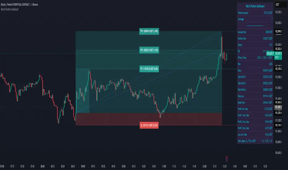
Smart Structure Pro - Market Structure & Smart Money Concepts═══════════════════════════════════════════════════════════════════════════════
SMART STRUCTURE PRO
═══════════════════════════════════════════════════════════════════════════════
A comprehensive market structure analysis tool that identifies institutional trading
patterns and smart money concepts for improved trade timing and decision-making.
═══════════════════════════════════════════════════════════════════════════════
📊 WHAT IT DOES
═══════════════════════════════════════════════════════════════════════════════
This indicator automatically detects and visualizes key market structure elements:
🔹 BOS (Break of Structure)
- Identifies trend continuation patterns
- Marks when price breaks above previous highs (bullish) or below previous lows (bearish)
- Confirms trend strength and momentum
🔹 CHoCH (Change of Character)
- Detects potential trend reversals
- Alerts when market structure shifts from bullish to bearish or vice versa
- Helps identify early reversal opportunities
🔹 Order Blocks
- Highlights institutional entry zones
- Identifies the last opposite candle before a structure break
- Shows areas where smart money likely entered positions
🔹 Fair Value Gaps (FVG)
- Detects price imbalances and inefficiencies
- Shows areas where price moved rapidly leaving gaps
- Often act as support/resistance when retested
🔹 Liquidity Zones
- Marks swing high and low levels
- Identifies areas where stop losses likely cluster
- Shows potential stop hunt and liquidity grab zones
═══════════════════════════════════════════════════════════════════════════════
🎯 HOW TO USE
═══════════════════════════════════════════════════════════════════════════════
BULLISH SETUP:
1. Wait for Bullish CHoCH (trend reversal signal) or BOS ↑ (continuation)
2. Look for price to pull back into an Order Block or Fair Value Gap
3. Enter long when price bounces from these zones
4. Place stop loss below the Order Block
5. Target the next liquidity zone or resistance level
BEARISH SETUP:
1. Wait for Bearish CHoCH (trend reversal signal) or BOS ↓ (continuation)
2. Look for price to retrace into an Order Block or Fair Value Gap
3. Enter short when price rejects from these zones
4. Place stop loss above the Order Block
5. Target the next liquidity zone or support level
DASHBOARD INTERPRETATION:
• Trend: Current market direction (Bullish/Bearish)
• Volume: Confirmation strength (High volume = stronger signals)
• Signal: Latest structure break detected
• Key High/Low: Critical levels for the current trend
• Position: Price location (Premium = expensive, Discount = cheap)
═══════════════════════════════════════════════════════════════════════════════
⚙️ SETTINGS GUIDE
═══════════════════════════════════════════════════════════════════════════════
STRUCTURE DETECTION:
• Pivot Length (Default: 10)
- Lower values = More signals but potentially weaker
- Higher values = Fewer signals but stronger/more reliable
- Recommended: 8-12 for intraday, 10-15 for higher timeframes
• Structure Line Extension
- Visual preference for how far lines extend
- Does not affect signal detection
SMART MONEY CONCEPTS:
• Order Block Extension: How long OB boxes remain visible
• FVG Extension: How long gap boxes remain visible
• Min FVG Size: Filter out small gaps (0 = show all)
- Set to 10-20% to reduce noise
- Set to 0 to see all gaps
VOLUME FILTER:
• Volume Confirmation (Recommended: ON)
- Filters weak signals without volume support
- Reduces false breakouts
• Volume Multiplier (Default: 1.5)
- Higher = Stricter filtering (fewer but stronger signals)
- Lower = More signals (but may include weak ones)
DISPLAY:
• Dashboard: Toggle information panel
• Trend Background: Subtle color tint showing current trend
• Dashboard Position: Choose corner placement
═══════════════════════════════════════════════════════════════════════════════
🔔 ALERTS
═══════════════════════════════════════════════════════════════════════════════
Available alert conditions:
✓ Bullish BOS - Uptrend continuation confirmed
✓ Bearish BOS - Downtrend continuation confirmed
✓ Bullish CHoCH - Reversal to uptrend detected
✓ Bearish CHoCH - Reversal to downtrend detected
✓ Structure Break - Any significant market structure change
To set up alerts:
1. Click the "⏰" alert icon
2. Select "Smart Structure Pro"
3. Choose your desired condition
4. Configure notification method
5. Click "Create"
═══════════════════════════════════════════════════════════════════════════════
⚠️ IMPORTANT DISCLOSURES
═══════════════════════════════════════════════════════════════════════════════
REPAINTING BEHAVIOR:
• Pivot points WILL repaint until confirmed (this is by design and unavoidable)
• Structure breaks (BOS/CHoCH) use CLOSED candles and do NOT repaint after confirmation
• Order Blocks and FVGs are drawn on confirmed signals and do NOT repaint
• All signals wait for candle close before triggering
BEST PRACTICES:
• Use on higher timeframes (15min+) for more reliable signals
• Combine with other analysis (support/resistance, volume profile, etc.)
• Wait for candle close confirmation before acting on signals
• Use proper risk management - this is not a standalone trading system
• Backtest on your preferred instrument and timeframe
PERFORMANCE:
• Limited to 100 boxes, 100 lines, 100 labels for optimal performance
• Older objects automatically removed as new ones appear
• Works on all markets (Forex, Crypto, Stocks, Indices, Commodities)
═══════════════════════════════════════════════════════════════════════════════
📚 CONCEPTS EXPLAINED
═══════════════════════════════════════════════════════════════════════════════
MARKET STRUCTURE:
Market structure refers to the pattern of price movements creating swing highs
and lows. Understanding structure helps identify trend direction and potential
reversal points.
SMART MONEY CONCEPTS:
These are trading techniques based on tracking institutional order flow and
understanding where large players (banks, funds, institutions) enter and exit
positions.
ORDER BLOCKS:
The last opposing candle before a strong directional move. Institutions often
leave unfilled orders in these zones, which can act as support/resistance when
price returns.
FAIR VALUE GAPS:
Areas where price moved so quickly that it left an imbalance. These gaps often
get "filled" as price returns to find equilibrium, creating trading opportunities.
═══════════════════════════════════════════════════════════════════════════════
🎓 EDUCATIONAL VALUE
═══════════════════════════════════════════════════════════════════════════════
This indicator helps traders:
✓ Understand market structure mechanics
✓ Identify institutional trading patterns
✓ Improve trade timing and entry precision
✓ Recognize trend continuation vs reversal
✓ Learn smart money concepts through visualization
═══════════════════════════════════════════════════════════════════════════════
📋 TECHNICAL DETAILS
═══════════════════════════════════════════════════════════════════════════════
• Version: 1.0.0
• Pine Script Version: 5
• Indicator Type: Overlay
• No Repainting: Structure breaks use confirmed candles
• Performance Optimized: Limited drawing objects
• Works On: All markets and timeframes
• Alerts: Yes, fully customizable
═══════════════════════════════════════════════════════════════════════════════
👤 AUTHOR
═══════════════════════════════════════════════════════════════════════════════
Created by: Zakaria Safri
Original Work: All code and concepts are original implementations
Based On: ICT (Inner Circle Trader) educational concepts
License: © 2024 Zakaria Safri - Personal Use Only
═══════════════════════════════════════════════════════════════════════════════
⚖️ DISCLAIMER
═══════════════════════════════════════════════════════════════════════════════
This indicator is for educational and informational purposes only. It does not
constitute financial advice. Trading involves substantial risk of loss. Past
performance does not guarantee future results. Always conduct your own research
and consult with a licensed financial advisor before making trading decisions.
The author is not responsible for any losses incurred from using this indicator.
═══════════════════════════════════════════════════════════════════════════════
If you find this indicator helpful, please:
👍 Like and favorite
⭐ Leave a review
📢 Share with other traders
💬 Comment with feedback or suggestions
Happy Trading! 📈

Yuki Leverage RR Calculator**YUKI LEVERAGE RR CALCULATOR**
A professional-grade risk/reward calculator for leveraged crypto or forex trades.
Instantly visualizes entry, stop loss, targets, leverage, and risk-to-reward ratios — helping you plan precise positions with confidence.
──────────────────────────────
**WHAT IT DOES**
Calculates position value, quantity, stop-loss price, liquidation estimate, and per-target profit.
Displays everything in an on-chart table with optional price tags and alerts.
──────────────────────────────
**KEY FEATURES**
• Long / Short toggle (only one active at a time)
• Leverage-aware position sizing based on Position Cost ($) and Leverage
• Dynamic Stop Loss: input % → auto price + $ risk
• Up to 3 Take-Profit Targets with scaling logic
• Instant R:R ratios per target
• Liquidation estimate (approximation only)
• ENTRY / SL / T1 / T2 / T3 / LIQ visual tags
• Dark/Light mode, adjustable table and tag size
• Built-in alerts for Targets and Stop Loss
──────────────────────────────
**INPUTS**
• Long or Short selection
• Entry Price, Stop Loss %
• Target 1 / Target 2 / Target 3 + Take Profit %
• Position Cost ($), Leverage
• Visual preferences: show/hide table, table corner, font size, tag offset, text size
──────────────────────────────
**TABLE OUTPUTS**
Position Info: Type, Entry, Position Cost, Leverage, Value
Risk Section: Stop Loss %, Stop Loss Price, Total Risk ($), Liquidation % & Price
Targets 1–3: Profit ($), R:R, Take Profit ($), Runner % or PnL
──────────────────────────────
**ALERTS**
• Target 1 Hit – when price crosses T1
• Target 2 Hit – when price crosses T2
• Target 3 Hit – when price crosses T3
• Stop Loss Hit – triggers based on direction
(Use TradingView Alerts → Condition → Indicator → select desired alert)
──────────────────────────────
**HOW TO USE**
1. Choose Long or Short
2. Enter Entry Price, Stop Loss %, Position Cost, and Leverage
3. Add Targets 1–3 with optional Take Profit %
4. Adjust visuals as desired
5. Monitor table + alerts for live trade planning
──────────────────────────────
**NOTES**
• Liquidation values are estimates only
• Fees, slippage, and funding not included
• Designed for educational and planning purposes
──────────────────────────────
⚠️ **DISCLAIMER**
For educational use only — not financial advice.
Trading leveraged products involves high risk of loss.
Always confirm calculations with your exchange and trade responsibly.
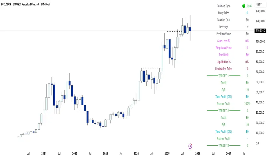
RSI Bollinger Bands [DCAUT]█ RSI Bollinger Bands
📊 ORIGINALITY & INNOVATION
The RSI Bollinger Bands indicator represents a meaningful advancement in momentum analysis by combining two proven technical tools: the Relative Strength Index (RSI) and Bollinger Bands. This combination addresses a significant limitation in traditional RSI analysis - the use of fixed overbought/oversold thresholds (typically 70/30) that fail to adapt to changing market volatility conditions.
Core Innovation:
Rather than relying on static threshold levels, this indicator applies Bollinger Bands statistical analysis directly to RSI values, creating dynamic zones that automatically adjust based on recent momentum volatility. This approach helps reduce false signals during low volatility periods while remaining sensitive to genuine extremes during high volatility conditions.
Key Enhancements Over Traditional RSI:
Dynamic Thresholds: Overbought/oversold zones adapt to market conditions automatically, eliminating the need for manual threshold adjustments across different instruments and timeframes
Volatility Context: Band width provides immediate visual feedback about momentum volatility, helping traders distinguish between stable trends and erratic movements
Reduced False Signals: During ranging markets, narrower bands filter out minor RSI fluctuations that would trigger traditional fixed-threshold signals
Breakout Preparation: Band squeeze patterns (similar to price-based BB) signal potential momentum regime changes before they occur
Self-Referencing Analysis: By measuring RSI against its own statistical behavior rather than arbitrary levels, the indicator provides more relevant context
📐 MATHEMATICAL FOUNDATION
Two-Stage Calculation Process:
Stage 1: RSI Calculation
RSI = 100 - (100 / (1 + RS))
where RS = Average Gain / Average Loss over specified period
The RSI normalizes price momentum into a bounded 0-100 scale, making it ideal for statistical band analysis.
Stage 2: Bollinger Bands on RSI
Basis = MA(RSI, BB Length)
Upper Band = Basis + (StdDev(RSI, BB Length) × Multiplier)
Lower Band = Basis - (StdDev(RSI, BB Length) × Multiplier)
Band Width = Upper Band - Lower Band
The Bollinger Bands measure RSI's standard deviation from its own moving average, creating statistically-derived dynamic zones.
Statistical Interpretation:
Under normal distribution assumptions with default 2.0 multiplier, approximately 95% of RSI values should fall within the bands
Band touches represent statistically significant momentum extremes relative to recent behavior
Band width expansion indicates increasing momentum volatility (strengthening trend or increasing uncertainty)
Band width contraction signals momentum consolidation and potential regime change preparation
📊 COMPREHENSIVE SIGNAL ANALYSIS
Visual Color Signals:
This indicator features dynamic color fills that highlight extreme momentum conditions:
Green Fill (Above Upper Band):
Appears when RSI breaks above the upper band, indicating exceptionally strong bullish momentum
Represents dynamic overbought zone - not necessarily a reversal signal but a warning of extreme conditions
In strong uptrends, green fills can persist as RSI "rides the band" - this indicates sustained momentum strength
Exit of green zone (RSI falling back below upper band) often signals initial momentum weakening
Red Fill (Below Lower Band):
Appears when RSI breaks below the lower band, indicating exceptionally weak bearish momentum
Represents dynamic oversold zone - potential reversal or continuation signal depending on trend context
In strong downtrends, red fills can persist as RSI "rides the band" - this indicates sustained selling pressure
Exit of red zone (RSI rising back above lower band) often signals initial momentum recovery
Position-Based Signals:
Upper Band Interactions:
RSI Touching Upper Band: Dynamic overbought condition - momentum is extremely strong relative to recent volatility, potential exhaustion or continuation depending on trend context
RSI Riding Upper Band: Sustained strong momentum, often seen in powerful trends, not necessarily an immediate reversal signal but warrants monitoring for exhaustion
RSI Crossing Below Upper Band: Initial momentum weakening signal, particularly significant if accompanied by price divergence
Lower Band Interactions:
RSI Touching Lower Band: Dynamic oversold condition - momentum is extremely weak relative to recent volatility, potential reversal or continuation of downtrend
RSI Riding Lower Band: Sustained weak momentum, common in strong downtrends, monitor for potential exhaustion
RSI Crossing Above Lower Band: Initial momentum strengthening signal, early indication of potential reversal or consolidation
Basis Line Signals:
RSI Above Basis: Bullish momentum regime - upward pressure dominant
RSI Below Basis: Bearish momentum regime - downward pressure dominant
Basis Crossovers: Momentum regime shifts, more significant when accompanied by band width changes
RSI Oscillating Around Basis: Balanced momentum, often indicates ranging market conditions
Volatility-Based Signals:
Band Width Patterns:
Narrow Bands (Squeeze): Momentum volatility compression, often precedes significant directional moves, similar to price coiling patterns
Expanding Bands: Increasing momentum volatility, indicates trend acceleration or growing uncertainty
Narrowest Band in 100 Bars: Extreme compression alert, high probability of upcoming volatility expansion
Advanced Pattern Recognition:
Divergence Analysis:
Bullish Divergence: Price makes lower lows while RSI touches or stays above previous lower band touch, suggests downward momentum weakening
Bearish Divergence: Price makes higher highs while RSI touches or stays below previous upper band touch, suggests upward momentum weakening
Hidden Bullish: Price makes higher lows while RSI makes lower lows at the lower band, indicates strong underlying bullish momentum
Hidden Bearish: Price makes lower highs while RSI makes higher highs at the upper band, indicates strong underlying bearish momentum
Band Walk Patterns:
Upper Band Walk: RSI consistently touching or staying near upper band indicates exceptionally strong trend, wait for clear break below basis before considering reversal
Lower Band Walk: RSI consistently at lower band signals very weak momentum, requires break above basis for reversal confirmation
🎯 STRATEGIC APPLICATIONS
Strategy 1: Mean Reversion Trading
Setup Conditions:
Market Type: Ranging or choppy markets with no clear directional trend
Timeframe: Works best on lower timeframes (5m-1H) or during consolidation phases
Band Characteristic: Normal to narrow band width
Entry Rules:
Long Entry: RSI touches or crosses below lower band, wait for RSI to start rising back toward basis before entry
Short Entry: RSI touches or crosses above upper band, wait for RSI to start falling back toward basis before entry
Confirmation: Use price action confirmation (candlestick reversal patterns) at band touches
Exit Rules:
Target: RSI returns to basis line or opposite band
Stop Loss: Fixed percentage or below recent swing low/high
Time Stop: Exit if position not profitable within expected timeframe
Strategy 2: Trend Continuation Trading
Setup Conditions:
Market Type: Clear trending market with higher highs/lower lows
Timeframe: Medium to higher timeframes (1H-Daily)
Band Characteristic: Expanding or wide bands indicating strong momentum
Entry Rules:
Long Entry in Uptrend: Wait for RSI to pull back to basis line or slightly below, enter when RSI starts rising again
Short Entry in Downtrend: Wait for RSI to rally to basis line or slightly above, enter when RSI starts falling again
Avoid Counter-Trend: Do not fade RSI at bands during strong trends (band walk patterns)
Exit Rules:
Trailing Stop: Move stop to break-even when RSI reaches opposite band
Trend Break: Exit when RSI crosses basis against trend direction with conviction
Band Squeeze: Reduce position size when bands start narrowing significantly
Strategy 3: Breakout Preparation
Setup Conditions:
Market Type: Consolidating market after significant move or at key technical levels
Timeframe: Any timeframe, but longer timeframes provide more reliable breakouts
Band Characteristic: Narrowest band width in recent 100 bars (squeeze alert)
Preparation Phase:
Identify band squeeze condition (bands at multi-period narrowest point)
Monitor price action for consolidation patterns (triangles, rectangles, flags)
Prepare bracket orders for both directions
Wait for band expansion to begin
Entry Execution:
Breakout Confirmation: Enter in direction of RSI band breakout (RSI breaks above upper band or below lower band)
Price Confirmation: Ensure price also breaks corresponding technical level
Volume Confirmation: Look for volume expansion supporting the breakout
Risk Management:
Stop Loss: Place beyond consolidation pattern opposite extreme
Position Sizing: Use smaller size due to false breakout risk
Quick Exit: Exit immediately if RSI returns inside bands within 1-3 bars
Strategy 4: Multi-Timeframe Analysis
Timeframe Selection:
Higher Timeframe: Daily or 4H for trend context
Trading Timeframe: 1H or 15m for entry signals
Confirmation Timeframe: 5m or 1m for precise entry timing
Analysis Process:
Trend Identification: Check higher timeframe RSI position relative to bands, trade only in direction of higher timeframe momentum
Setup Formation: Wait for trading timeframe RSI to show pullback to basis in trending direction
Entry Timing: Use confirmation timeframe RSI band touch or crossover for precise entry
Alignment Confirmation: All timeframes should show RSI moving in same direction for highest probability setups
📋 DETAILED PARAMETER CONFIGURATION
RSI Source:
Close (Default): Standard price point, balances responsiveness and reliability
HL2: Reduces noise from intrabar volatility, provides smoother RSI values
HLC3 or OHLC4: Further smoothing for very choppy markets, slower to respond but more stable
Volume-Weighted: Consider using VWAP or volume-weighted prices for additional liquidity context
RSI Length Parameter:
Shorter Periods (5-10): More responsive but generates more signals, suitable for scalping or very active trading, higher noise level
Standard (14): Default and most widely used setting, proven balance between responsiveness and reliability, recommended starting point
Longer Periods (21-30): Smoother momentum measurement, fewer but potentially more reliable signals, better for swing trading or position trading
Optimization Note: Test across different market regimes, optimal length often varies by instrument volatility characteristics
RSI MA Type Parameter:
RMA (Default): Wilder's original smoothing method, provides traditional RSI behavior with balanced lag, most widely recognized and tested, recommended for standard technical analysis
EMA: Exponential smoothing gives more weight to recent values, faster response to momentum changes, suitable for active trading and trending markets, reduces lag compared to RMA
SMA: Simple average treats all periods equally, smoothest output with highest lag, best for filtering noise in choppy markets, useful for long-term position analysis
WMA: Weighted average emphasizes recent data less aggressively than EMA, middle ground between SMA and EMA characteristics, balanced responsiveness for swing trading
Advanced Options: Full access to 25+ moving average types including HMA (reduced lag), DEMA/TEMA (enhanced responsiveness), KAMA/FRAMA (adaptive behavior), T3 (smoothness), Kalman Filter (optimal estimation)
Selection Guide: RMA for traditional analysis and backtesting consistency, EMA for faster signals in trending markets, SMA for stability in ranging markets, adaptive types (KAMA/FRAMA) for varying volatility regimes
BB Length Parameter:
Short Length (10-15): Tighter bands that react quickly to RSI changes, more frequent band touches, suitable for active trading styles
Standard (20): Balanced approach providing meaningful statistical context without excessive lag
Long Length (30-50): Smoother bands that filter minor RSI fluctuations, captures only significant momentum extremes, fewer but higher quality signals
Relationship to RSI Length: Consider BB Length greater than RSI Length for cleaner signals
BB MA Type Parameter:
SMA (Default): Standard Bollinger Bands calculation using simple moving average for basis line, treats all periods equally, widely recognized and tested approach
EMA: Exponential smoothing for basis line gives more weight to recent RSI values, creates more responsive bands that adapt faster to momentum changes, suitable for trending markets
RMA: Wilder's smoothing provides consistent behavior aligned with traditional RSI when using RMA for both RSI and BB calculations
WMA: Weighted average for basis line balances recent emphasis with historical context, middle ground between SMA and EMA responsiveness
Advanced Options: Full access to 25+ moving average types for basis calculation, including HMA (reduced lag), DEMA/TEMA (enhanced responsiveness), KAMA/FRAMA (adaptive to volatility changes)
Selection Guide: SMA for standard Bollinger Bands behavior and backtesting consistency, EMA for faster band adaptation in dynamic markets, matching RSI MA type creates unified smoothing behavior
BB Multiplier Parameter:
Conservative (1.5-1.8): Tighter bands resulting in more frequent touches, useful in low volatility environments, higher signal frequency but potentially more false signals
Standard (2.0): Default setting representing approximately 95% confidence interval under normal distribution, widely accepted statistical threshold
Aggressive (2.5-3.0): Wider bands capturing only extreme momentum conditions, fewer but potentially more significant signals, reduces false signals in high volatility
Adaptive Approach: Consider adjusting multiplier based on instrument characteristics, lower multiplier for stable instruments, higher for volatile instruments
Parameter Optimization Workflow:
Start with default parameters (RSI:14, BB:20, Mult:2.0)
Test across representative sample period including different market regimes
Adjust RSI length based on desired responsiveness vs stability tradeoff
Tune BB length to match your typical holding period
Modify multiplier to achieve desired signal frequency
Validate on out-of-sample data to avoid overfitting
Document optimal parameters for different instruments and timeframes
Reference Levels Display:
Enabled (Default): Shows traditional 30/50/70 levels for comparison with dynamic bands, helps visualize the adaptive advantage
Disabled: Cleaner chart focusing purely on dynamic zones, reduces visual clutter for experienced users
Educational Value: Keeping reference levels visible helps understand how dynamic bands differ from fixed thresholds across varying market conditions
📈 PERFORMANCE ANALYSIS & COMPETITIVE ADVANTAGES
Comparison with Traditional RSI:
Fixed Threshold RSI Limitations:
In ranging low-volatility markets: RSI rarely reaches 70/30, missing tradable extremes
In trending high-volatility markets: RSI frequently breaks through 70/30, generating excessive false reversal signals
Across different instruments: Same thresholds applied to volatile crypto and stable forex pairs produce inconsistent results
Threshold Adjustment Problem: Manually changing thresholds for different conditions is subjective and lagging
RSI Bollinger Bands Advantages:
Automatic Adaptation: Bands adjust to current volatility regime without manual intervention
Consistent Logic: Same statistical approach works across different instruments and timeframes
Reduced False Signals: Band width filtering helps distinguish meaningful extremes from noise
Additional Information: Band width provides volatility context missing in standard RSI
Objective Extremes: Statistical basis (standard deviations) provides objective extreme definition
Comparison with Price-Based Bollinger Bands:
Price BB Characteristics:
Measures absolute price volatility
Affected by large price gaps and outliers
Band position relative to price not normalized
Difficult to compare across different price scales
RSI BB Advantages:
Normalized Scale: RSI's 0-100 bounds make band interpretation consistent across all instruments
Momentum Focus: Directly measures momentum extremes rather than price extremes
Reduced Gap Impact: RSI calculation smooths price gaps impact on band calculations
Comparable Analysis: Same RSI BB appearance across stocks, forex, crypto enables consistent strategy application
Performance Characteristics:
Signal Quality:
Higher Signal-to-Noise Ratio: Dynamic bands help filter RSI oscillations that don't represent meaningful extremes
Context-Aware Alerts: Band width provides volatility context helping traders adjust position sizing and stop placement
Reduced Whipsaws: During consolidations, narrower bands prevent premature signals from minor RSI movements
Responsiveness:
Adaptive Lag: Band calculation introduces some lag, but this lag is adaptive to current conditions rather than fixed
Faster Than Manual Adjustment: Automatic band adjustment is faster than trader's ability to manually modify thresholds
Balanced Approach: Combines RSI's inherent momentum lag with BB's statistical smoothing for stable yet responsive signals
Versatility:
Multi-Strategy Application: Supports both mean reversion (ranging markets) and trend continuation (trending markets) approaches
Universal Instrument Coverage: Works effectively across equities, forex, commodities, cryptocurrencies without parameter changes
Timeframe Agnostic: Same interpretation applies from 1-minute charts to monthly charts
Limitations and Considerations:
Known Limitations:
Dual Lag Effect: Combines RSI's momentum lag with BB's statistical lag, making it less suitable for very short-term scalping
Requires Volatility History: Needs sufficient bars for BB calculation, less effective immediately after major regime changes
Statistical Assumptions: Assumes RSI values are somewhat normally distributed, extreme trending conditions may violate this
Not a Standalone System: Like all indicators, should be combined with price action analysis and risk management
Optimal Use Cases:
Best for swing trading and position trading timeframes
Most effective in markets with alternating volatility regimes
Ideal for traders who use multiple instruments and timeframes
Suitable for systematic trading approaches requiring consistent logic
Suboptimal Conditions:
Very low timeframes (< 5 minutes) where lag becomes problematic
Instruments with extreme volatility spikes (gap-prone markets)
Markets in strong persistent trends where mean reversion rarely occurs
Periods immediately following major structural changes (new trading regime)
USAGE NOTES
This indicator is designed for technical analysis and educational purposes to help traders understand the interaction between momentum measurement and statistical volatility bands. The RSI Bollinger Bands has limitations and should not be used as the sole basis for trading decisions.
Important Considerations:
No Predictive Guarantee: Past band touches and patterns do not guarantee future price behavior
Market Regime Dependency: Indicator performance varies significantly between trending and ranging market conditions
Complementary Analysis Required: Should be used alongside price action, support/resistance levels, and fundamental analysis
Risk Management Essential: Always use proper position sizing, stop losses, and risk controls regardless of signal quality
Parameter Sensitivity: Different instruments and timeframes may require parameter optimization for optimal results
Continuous Monitoring: Band characteristics change with market conditions, requiring ongoing assessment
Recommended Supporting Analysis:
Price structure analysis (support/resistance, trend lines)
Volume confirmation for breakout signals
Multiple timeframe alignment
Market context awareness (news events, session times)
Correlation analysis with related instruments
The indicator aims to provide adaptive momentum analysis that adjusts to changing market volatility, but traders must apply sound judgment, proper risk management, and comprehensive market analysis in their decision-making process.

Quantum State Superposition Indicator (QSSI)Quantum State Superposition Indicator (QSSI) - Where Physics Meets Finance
The Quantum Revolution in Market Analysis
After months of research into quantum mechanics and its applications to financial markets, I'm thrilled to present the Quantum State Superposition Indicator (QSSI) - a groundbreaking approach that models price action through the lens of quantum physics. This isn't just another technical indicator; it's a paradigm shift in how we understand market behavior.
The Theoretical Foundation
Quantum Superposition in Markets
In quantum mechanics, particles exist in multiple states simultaneously until observed. Similarly, markets exist in a superposition of potential states (bullish, bearish, neutral) until a significant volume event "collapses" the wave function into a definitive direction.
The mathematical framework:
Wave Function (Ψ): Represents the market's quantum state as a weighted sum of all possible states:
Ψ = Σ(αᵢ × Sᵢ)
Where αᵢ are probability amplitudes and Sᵢ are individual quantum states.
Probability Amplitudes: Calculated using the Born rule, normalized so Σ|αᵢ|² = 1
Observation Operator: Volume/Average Volume ratio determines observation strength
The Five Quantum States
Momentum State: Short-term price velocity (EMA of returns)
Mean Reversion State: Deviation from equilibrium (normalized z-score)
Volatility Expansion State: ATR relative to historical average
Trend Continuation State: Long-term price positioning
Chaos State: Volatility of volatility (market uncertainty)
Each state contributes to the overall wave function based on current market conditions.
Wave Function Collapse
When volume exceeds the observation threshold (default 1.5x average), the wave function "collapses," committing the market to a direction. This models how institutional volume forces markets out of uncertainty into trending states.
Collapse Detection Formula:
Collapse = Volume > (Threshold × Average Volume)
Direction = Sign(Ψ) at collapse moment
Advanced Quantum Concepts
Heisenberg Uncertainty Principle
The indicator calculates market uncertainty as the product of price and momentum
uncertainties:
ΔP × ΔM = ℏ (market uncertainty constant)
This manifests as dynamic uncertainty bands that widen during unstable periods.
Quantum Tunneling
Calculates the probability of price "tunneling" through resistance/support barriers:
P(tunnel) = e^(-2×|barrier_height|×√coherence_length)
Unlike classical technical analysis, this gives probability of breakouts before they occur.
Entanglement
Measures the quantum correlation between price and volume:
Entanglement = |Correlation(Price, Volume, lookback)|
High entanglement suggests coordinated institutional activity.
Decoherence
When market states lose quantum properties and behave classically:
Decoherence = 1 - Σ(amplitude²)
Indicates trend emergence from quantum uncertainty.
Visual Innovation
Probability Clouds
Three-tier probability distributions visualize market uncertainty:
Inner Cloud (68%): One standard deviation - most likely price range
Middle Cloud (95%): Two standard deviations - probable extremes
Outer Cloud (99.7%): Three standard deviations - tail risk zones
Cloud width directly represents market uncertainty - wider clouds signal higher entropy states.
Quantum State Visualization
Colored dots represent individual quantum states:
Green: Momentum state strength
Red: Mean reversion state strength
Yellow: Volatility state strength
Dot brightness indicates amplitude (influence) of each state.
Collapse Events
Aqua Diamonds (Above): Bullish collapse - upward commitment
Pink Diamonds (Below): Bearish collapse - downward commitment
These mark precise moments when markets exit superposition.
Implementation Details
Core Calculations
Feature Extraction: Normalize price returns, volume ratios, and volatility measures
State Calculation: Compute each quantum state's value
Amplitude Assignment: Weight states by market conditions and observation strength
Wave Function: Sum weighted states for final market quantum state
Visualization: Transform quantum values to price space for display
Performance Optimization
- Efficient array operations for state calculations
- Single-pass normalization algorithms
- Optimized correlation calculations for entanglement
- Smart label management to prevent visual clutter
Trading Applications:
Signal Generation
Bullish Signals:
- Positive wave function during collapse
- High tunneling probability at support
- Coherent market state with bullish bias
Bearish Signals:
- Negative wave function during collapse
- High tunneling probability at resistance
- Decoherent state transitioning bearish
Risk Management
Uncertainty-Based Position Sizing:
Narrow clouds: Normal position size
Wide clouds: Reduced position size
Extreme uncertainty: Stay flat
Quantum Stop Losses:
- Place stops outside probability clouds
- Adjust for Heisenberg uncertainty
- Respect quantum tunneling levels
Market Regime Recognition
Quantum Coherent (Superposed):
- Market in multiple states
- Avoid directional trades
- Prepare for collapse
Quantum Decoherent (Classical):
-Clear trend emergence
- Follow directional signals
- Traditional analysis applies
Advanced Features
Adaptive Dashboards
Quantum State Panel: Real-time wave function, dominant state, and coherence status
Performance Metrics: Win rate, signal frequency, and regime analysis
Information Guide: Comprehensive explanation of all quantum concepts
- All dashboards feature adjustable sizing for different screen resolutions.
Multi-Timeframe Quantum Analysis
The indicator adapts to any timeframe:
Scalping (1-5m): Short coherence length, sensitive thresholds
Day Trading (15m-1H): Balanced parameters
Swing Trading (4H-1D): Long coherence, stable states
Alert System
Sophisticated alerts for:
- Wave function collapse events
- Decoherence transitions
- High tunneling probability
- Strong entanglement detection
Originality & Innovation
This indicator introduces several firsts:
Quantum Superposition: First to model markets as quantum systems
Wave Function Collapse: Original volume-triggered state commitment
Tunneling Probability: Novel breakout prediction method
Entanglement Metrics: Unique price-volume quantum correlation
Probability Clouds: Revolutionary uncertainty visualization
Development Journey
Creating QSSI required:
- Deep study of quantum mechanics principles
- Translation of physics equations to market context
- Extensive backtesting across multiple markets
- UI/UX optimization for trader accessibility
- Performance optimization for real-time calculation
- The result bridges cutting-edge physics with practical trading.
Best Practices
Parameter Optimization
Quantum States (2-5):
- 2-3 for simple markets (forex majors)
- 4-5 for complex markets (indices, crypto)
Coherence Length (10-50):
- Lower for fast markets
- Higher for stable markets
Observation Threshold (1.0-3.0):
- Lower for active markets
- Higher for thin markets
Signal Confirmation
Always confirm quantum signals with:
- Market structure (support/resistance)
- Volume patterns
- Correlated assets
- Fundamental context
Risk Guidelines
- Never risk more than 2% per trade
- Respect probability cloud boundaries
- Exit on decoherence shifts
- Scale with confidence levels
Educational Value
QSSI teaches advanced concepts:
- Quantum mechanics applications
- Probability theory
- Non-linear dynamics
- Risk management
- Market microstructure
Perfect for traders seeking deeper market understanding.
Disclaimer
This indicator is for educational and research purposes only. While quantum mechanics provides a fascinating framework for market analysis, no indicator can predict future prices with certainty. The probabilistic nature of both quantum mechanics and markets means outcomes are inherently uncertain.
Always use proper risk management, conduct thorough analysis, and never risk more than you can afford to lose. Past performance does not guarantee future results.
Conclusion
The Quantum State Superposition Indicator represents a revolutionary approach to market analysis, bringing institutional-grade quantum modeling to retail traders. By viewing markets through the lens of quantum mechanics, we gain unique insights into uncertainty, probability, and state transitions that classical indicators miss.
Whether you're a physicist interested in finance or a trader seeking cutting-edge tools, QSSI opens new dimensions in market analysis.
"The market, like Schrödinger's cat, exists in multiple states until observed through volume."
* As you may have noticed, the past two indicators I've released (Lorentzian Classification and Quantum State Superposition) are designed with strategy implementation in mind. I'm currently developing a stable execution platform that's completely unique and moves away from traditional ATR-based position sizing and stop loss systems. I've found ATR-based approaches to be unreliable in volatile markets and regime transitions - they often lag behind actual market conditions and can lead to premature exits or oversized positions during volatility spikes.
The goal is to create something that adapts to market conditions in real-time using the quantum and relativistic principles we've been exploring. Hopefully I'll have something groundbreaking to share soon. Stay tuned!
Trade with quantum insight. Trade with QSSI .
— Dskyz , for DAFE Trading Systems
